arviz.plot_density

arviz.plot_density(data, group='posterior', data_labels=None, var_names=None, filter_vars=None, combine_dims=None, transform=None, hdi_prob=None, point_estimate='auto', colors='cycle', outline=True, hdi_markers='', shade=0.0, bw='default', circular=False, grid=None, figsize=None, textsize=None, labeller=None, ax=None, backend=None, backend_kwargs=None, show=None)

Generate KDE plots for continuous variables and histograms for discrete ones.

Plots are truncated at their 100*(1-alpha)% highest density intervals. Plots are grouped per variable and colors assigned to models.

Parameters:

dataInferenceData or iterable of InferenceData

Any object that can be converted to an arviz.InferenceData object, or an Iterator returning a sequence of such objects. Refer to documentation of arviz.convert_to_dataset() for details.

group{“posterior”, “prior”}, default “posterior”

Specifies which InferenceData group should be plotted. If “posterior”, then the values in posterior_predictive group are compared to the ones in observed_data, if “prior” then the same comparison happens, but with the values in prior_predictive group.

data_labelslist of str, default None

List with names for the datasets passed as “data.” Useful when plotting more than one dataset. Must be the same shape as the data parameter.

var_nameslist of str, optional

List of variables to plot. If multiple datasets are supplied and var_names is not None, will print the same set of variables for each dataset. Defaults to None, which results in all the variables being plotted.

filter_vars{None, “like”, “regex”}, default None

If None (default), interpret var_names as the real variables names. If “like”, interpret var_names as substrings of the real variables names. If “regex”, interpret var_names as regular expressions on the real variables names. See this section for usage examples.

combine_dimsset_like of str, optional

List of dimensions to reduce. Defaults to reducing only the “chain” and “draw” dimensions. See this section for usage examples.

transformcallable()

Function to transform data (defaults to None i.e. the identity function).

hdi_probfloat, default 0.94

Probability for the highest density interval. Should be in the interval (0, 1]. See this section for usage examples.

point_estimatestr, optional

Plot point estimate per variable. Values should be ‘mean’, ‘median’, ‘mode’ or None. Defaults to ‘auto’ i.e. it falls back to default set in rcParams.

colorsstr or list of str, optional

List with valid matplotlib colors, one color per model. Alternative a string can be passed. If the string is cycle, it will automatically choose a color per model from matplotlib’s cycle. If a single color is passed, e.g. ‘k’, ‘C2’ or ‘red’ this color will be used for all models. Defaults to cycle.

outlinebool, default True

Use a line to draw KDEs and histograms.

hdi_markersstr

A valid matplotlib.markers like ‘v’, used to indicate the limits of the highest density interval. Defaults to empty string (no marker).

shadefloat, default 0

Alpha blending value for the shaded area under the curve, between 0 (no shade) and 1 (opaque).

bwfloat or str, optional

If numeric, indicates the bandwidth and must be positive. If str, indicates the method to estimate the bandwidth and must be one of “scott”, “silverman”, “isj” or “experimental” when circular is False and “taylor” (for now) when circular is True. Defaults to “default” which means “experimental” when variable is not circular and “taylor” when it is.

circularbool, default False

If True, it interprets the values passed are from a circular variable measured in radians and a circular KDE is used. Only valid for 1D KDE.

gridtuple, optional

Number of rows and columns. Defaults to None, the rows and columns are automatically inferred. See this section for usage examples.

figsize(float, float), optional

Figure size. If None it will be defined automatically.

textsizefloat, optional

Text size scaling factor for labels, titles and lines. If None it will be autoscaled based on figsize.

labellerLabeller, optional

Class providing the method make_label_vert to generate the labels in the plot titles. Read the Label guide for more details and usage examples.

ax2D array_like of matplotlib Axes or Bokeh Figure, optional

A 2D array of locations into which to plot the densities. If not supplied, ArviZ will create its own array of plot areas (and return it).

backend{“matplotlib”, “bokeh”}, default “matplotlib”

Select plotting backend.

backend_kwargsdict, optional

These are kwargs specific to the backend being used, passed to matplotlib.pyplot.subplots() or bokeh.plotting.figure. For additional documentation check the plotting method of the backend.

showbool, optional

Call backend show function.

Returns:

axes2D ndarray of matplotlib Axes or Bokeh Figure

See also

plot_dist

Plot distribution as histogram or kernel density estimates.

plot_posterior

Plot Posterior densities in the style of John K. Kruschke’s book.

Examples

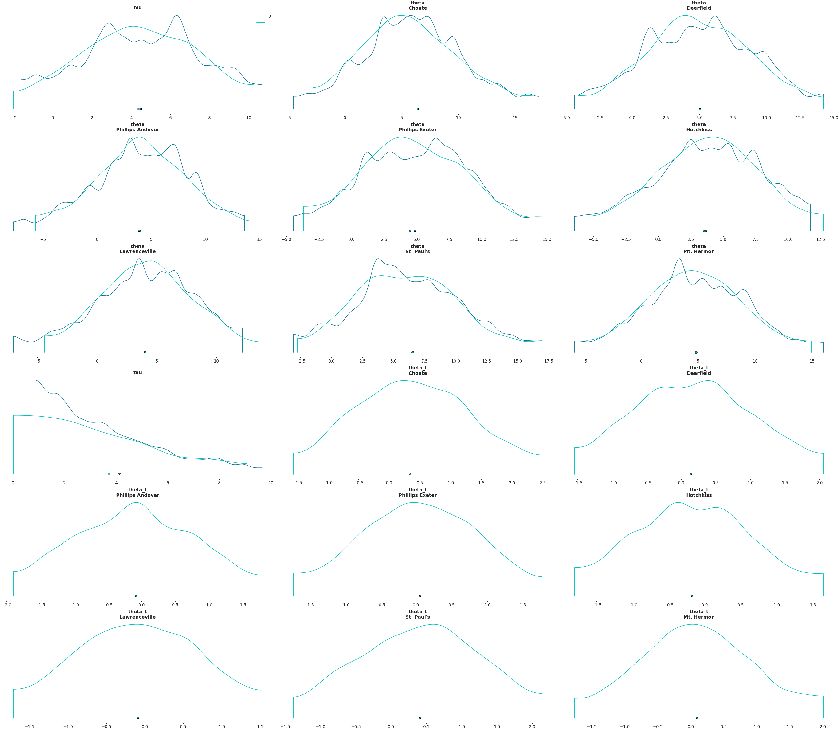
Plot default density plot

>>> import arviz as az
>>> centered = az.load_arviz_data('centered_eight')
>>> non_centered = az.load_arviz_data('non_centered_eight')
>>> az.plot_density([centered, non_centered])

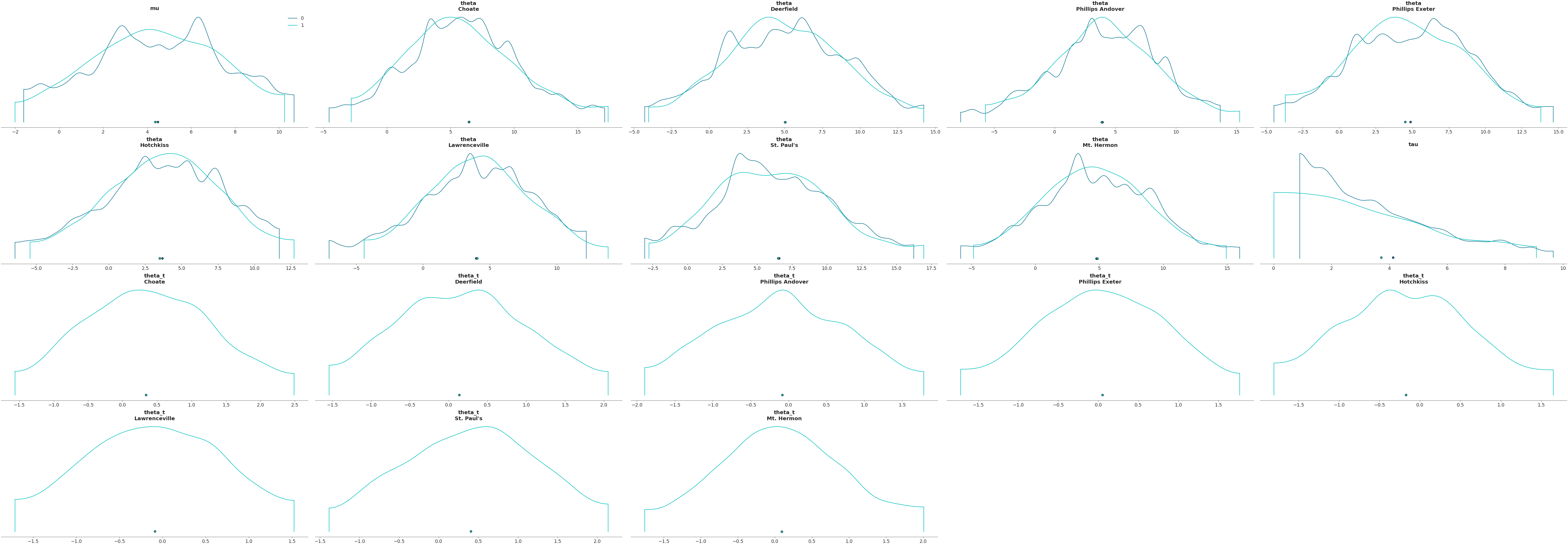
Plot variables in a 4x5 grid

>>> az.plot_density([centered, non_centered], grid=(4, 5))

Plot subset variables by specifying variable name exactly

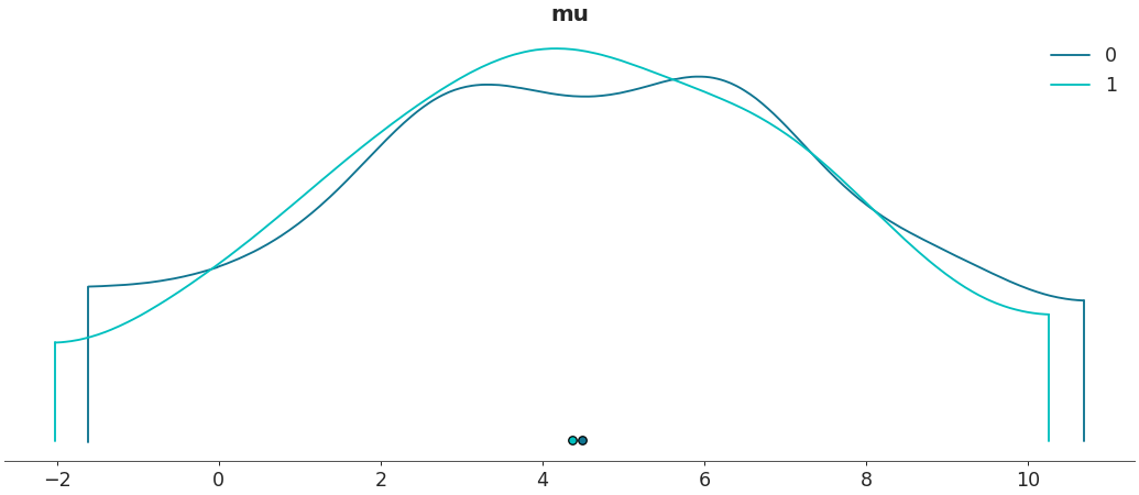
>>> az.plot_density([centered, non_centered], var_names=["mu"])

Plot a specific az.InferenceData group

>>> az.plot_density([centered, non_centered], var_names=["mu"], group="prior")

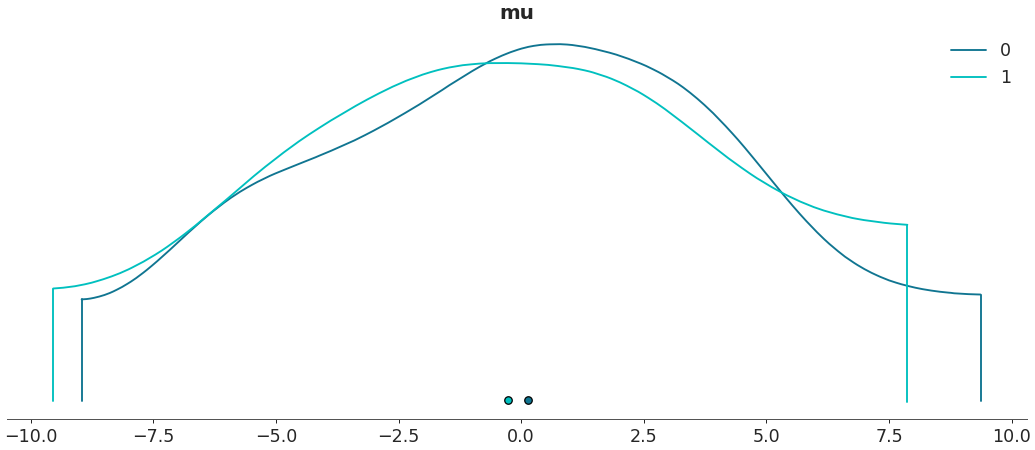
Specify highest density interval

>>> az.plot_density([centered, non_centered], var_names=["mu"], hdi_prob=.5)

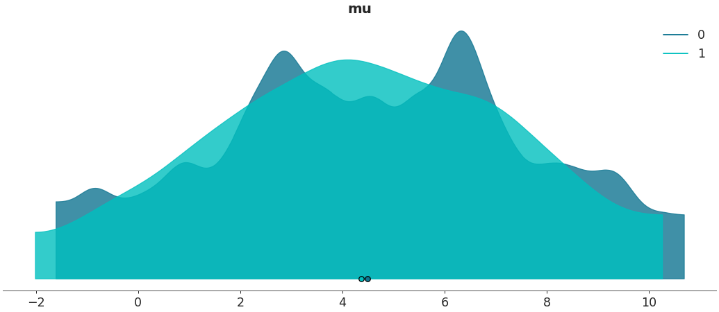
Shade plots and/or remove outlines

>>> az.plot_density([centered, non_centered], var_names=["mu"], outline=False, shade=.8)

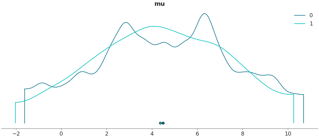
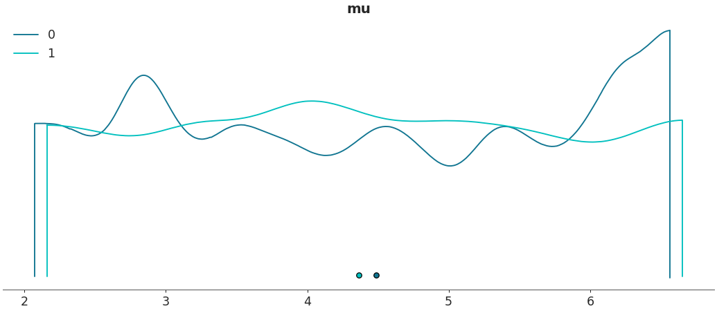
Specify binwidth for kernel density estimation

>>> az.plot_density([centered, non_centered], var_names=["mu"], bw=.9)