Label guide#
Basic labelling#
All ArviZ plotting functions and some stats functions can take an optional labeller argument.
By default, labels show the variable name.
Multidimensional variables also show the coordinate value.
Example: Default labelling#
In [1]: import arviz as az
   ...: schools = az.load_arviz_data("centered_eight")
   ...: az.summary(schools)
   ...:
Out[1]:
                        mean   sd eti89_lb  ... r_hat  mcse_mean  mcse_sd
mu                       4.2  3.3     -1.2  ...  1.03       0.21     0.14
theta[Choate]            6.4  5.9     -1.7  ...  1.01       0.25     0.24
theta[Deerfield]           5  4.9       -3  ...  1.01       0.21     0.19
theta[Phillips Andover]  3.4  5.4     -5.7  ...  1.01       0.23     0.21
theta[Phillips Exeter]   4.8  5.2     -3.1  ...  1.01       0.21     0.21
theta[Hotchkiss]         3.5  4.8     -4.3  ...  1.02       0.25      0.2
theta[Lawrenceville]     3.7  5.2     -4.4  ...  1.01       0.22     0.21
theta[St. Paul's]        6.5  5.2       -1  ...  1.01       0.22     0.19
theta[Mt. Hermon]        4.8  5.7     -3.8  ...  1.01       0.24     0.25
tau                      4.3    3      1.3  ...  1.03       0.22      0.3

[10 rows x 9 columns]
ArviZ supports label based indexing powered by xarray. Through label based indexing, you can use labels to plot a subset of selected variables.
Example: Label based indexing#
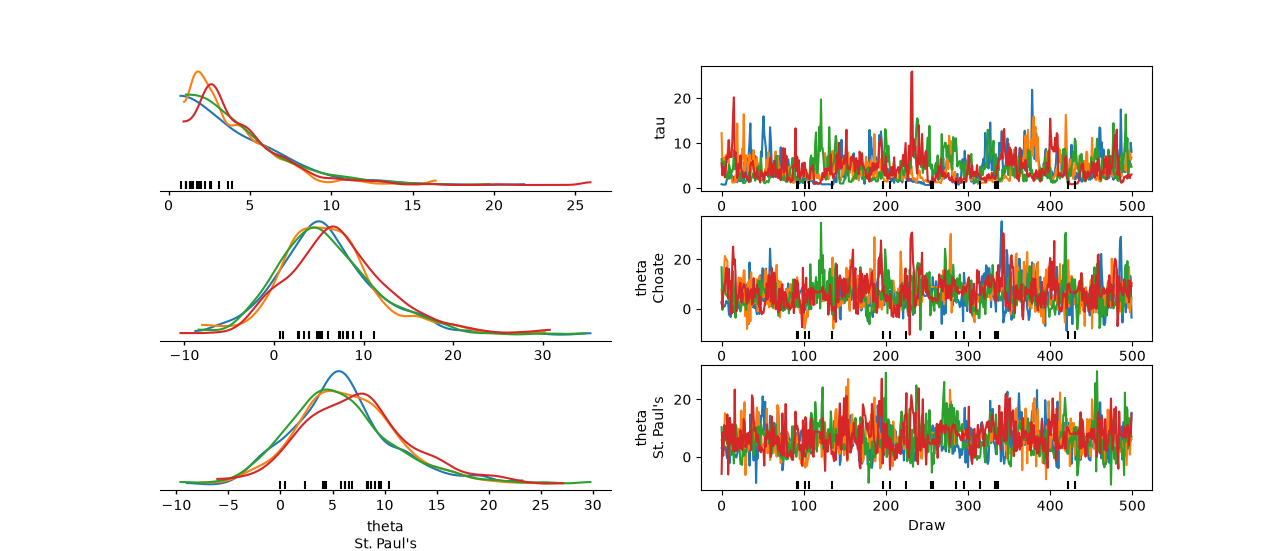
For a case where the coordinate values shown for the theta variable coordinate to the school dimension,
you can indicate ArviZ to plot tau by including it in the var_names argument to inspect its 1.03 rhat() value.
To inspect the theta values for the Choate and St. Paul's coordinates, you can include theta in var_names and use the coords argument to select only these two coordinate values.
You can generate this plot with the following command:
In [2]: az.plot_trace_dist(
   ...:     schools,
   ...:     var_names=["tau", "theta"],
   ...:     coords={"school": ["Choate", "St. Paul's"]},
   ...:     compact=False
   ...: );
   ...:

Using the above command, you can now identify issues for low tau values.
Example: Using the labeller argument#
You can use the labeller argument to customize labels.
Unlike the default labels that show theta, not \(\theta\) (generated from $\theta$ using \(\LaTeX\)), the labeller argument presents the labels with proper math notation.
You can use MapLabeller to rename the variable theta to $\theta$, as shown in the following example:
In [3]: import arviz.labels as azl
   ...: labeller = azl.MapLabeller(var_name_map={"theta": r"$\theta$"})
   ...: coords = {"school": ["Deerfield", "Hotchkiss", "Lawrenceville"]}
   ...:
---------------------------------------------------------------------------
ModuleNotFoundError                       Traceback (most recent call last)
Cell In[3], line 1
----> 1 import arviz.labels as azl
      2 labeller = azl.MapLabeller(var_name_map={"theta": r"$\theta$"})
      3 coords = {"school": ["Deerfield", "Hotchkiss", "Lawrenceville"]}

ModuleNotFoundError: No module named 'arviz.labels'

In [4]: az.plot_dist(
   ...:     schools,
   ...:     var_names="theta",
   ...:     coords=coords,
   ...:     labeller=labeller
   ...: );
   ...:
---------------------------------------------------------------------------
NameError                                 Traceback (most recent call last)
Cell In[4], line 4
      1 az.plot_dist(
      2     schools,
      3     var_names="theta",
----> 4     coords=coords,
      5     labeller=labeller
      6 );

NameError: name 'coords' is not defined
See also
For a list of labellers available in ArviZ, see the the API reference page.
Sorting labels#
ArviZ allows labels to be sorted in two ways:
Using the arguments passed to ArviZ plotting functions
Sorting the underlying
xarray.Dataset
The first option is more suitable for single time ordering whereas the second option is more suitable for sorting plots consistently.
Note
Both ways are limited.
Multidimensional variables can not be separated.
For example, it is possible to sort theta, mu, or tau in any order, and within theta to sort the schools in any order, but it is not possible to sort half of the schools, then mu and tau and then the rest of the schools.
Sorting variable names#
In [5]: var_order = ["theta", "mu", "tau"]
For variable names to appear sorted when calling ArviZ functions, pass a sorted list of the variable names.
In [6]: az.summary(schools, var_names=var_order)
Out[6]:
                        mean   sd eti89_lb  ... r_hat  mcse_mean  mcse_sd
theta[Choate]            6.4  5.9     -1.7  ...  1.01       0.25     0.24
theta[Deerfield]           5  4.9       -3  ...  1.01       0.21     0.19
theta[Phillips Andover]  3.4  5.4     -5.7  ...  1.01       0.23     0.21
theta[Phillips Exeter]   4.8  5.2     -3.1  ...  1.01       0.21     0.21
theta[Hotchkiss]         3.5  4.8     -4.3  ...  1.02       0.25      0.2
theta[Lawrenceville]     3.7  5.2     -4.4  ...  1.01       0.22     0.21
theta[St. Paul's]        6.5  5.2       -1  ...  1.01       0.22     0.19
theta[Mt. Hermon]        4.8  5.7     -3.8  ...  1.01       0.24     0.25
mu                       4.2  3.3     -1.2  ...  1.03       0.21     0.14
tau                      4.3    3      1.3  ...  1.03       0.22      0.3

[10 rows x 9 columns]
In xarray, subsetting the Dataset with a sorted list of variable names will order the Dataset.
In [7]: schools.posterior = schools.posterior[var_order]
   ...: az.summary(schools)
   ...:
---------------------------------------------------------------------------
NotImplementedError                       Traceback (most recent call last)
Cell In[7], line 1
----> 1 schools.posterior = schools.posterior[var_order]
      2 az.summary(schools)

File ~/checkouts/readthedocs.org/user_builds/arviz/envs/stable/lib/python3.12/site-packages/xarray/core/datatree.py:1009, in DataTree.__getitem__(self, key)
   1006     return self._get_item(path)
   1007 elif utils.is_list_like(key):
   1008     # iterable of variable names
-> 1009     raise NotImplementedError(
   1010         "Selecting via tags is deprecated, and selecting multiple items should be "
   1011         "implemented via .subset"
   1012     )
   1013 else:
   1014     raise ValueError(f"Invalid format for key: {key}")

NotImplementedError: Selecting via tags is deprecated, and selecting multiple items should be implemented via .subset
Sorting coordinate values#
For sorting coordinate values, first, define the order, then store it, and use the result to sort the coordinate values. You can define the order by creating a list manually or by using xarray objects as illustrated in the below example “Sorting out the schools by mean”.
Example: Sorting the schools by mean#
Locate the means of each school by using the following command:
In [8]: school_means = schools.posterior["theta"].mean(("chain", "draw"))
   ...: school_means
   ...:
Out[8]:
<xarray.DataArray 'theta' (school: 8)> Size: 64B
array([6.42044255, 4.95449743, 3.42293245, 4.7535654 , 3.45303468,
       3.66295895, 6.50522692, 4.81977956])
Coordinates:
  * school   (school) <U16 512B 'Choate' 'Deerfield' ... 'Mt. Hermon'
You can use the
DataArrayresult to sort the coordinate values fortheta.
There are two ways of sorting:
Arviz args
xarray
Sort the coordinate values to pass them as a coords argument and choose the order of the rows.
In [9]: sorted_schools = schools.posterior["school"].sortby(school_means)
   ...: az.summary(schools, var_names="theta", coords={"school": sorted_schools})
   ...:
Out[9]:
                        mean   sd eti89_lb  ... r_hat  mcse_mean  mcse_sd
theta[Phillips Andover]  3.4  5.4     -5.7  ...  1.01       0.23     0.21
theta[Hotchkiss]         3.5  4.8     -4.3  ...  1.02       0.25      0.2
theta[Lawrenceville]     3.7  5.2     -4.4  ...  1.01       0.22     0.21
theta[Phillips Exeter]   4.8  5.2     -3.1  ...  1.01       0.21     0.21
theta[Mt. Hermon]        4.8  5.7     -3.8  ...  1.01       0.24     0.25
theta[Deerfield]           5  4.9       -3  ...  1.01       0.21     0.19
theta[Choate]            6.4  5.9     -1.7  ...  1.01       0.25     0.24
theta[St. Paul's]        6.5  5.2       -1  ...  1.01       0.22     0.19

[8 rows x 9 columns]
You can use the sortby() method to order our coordinate values directly at the source.
In [10]: schools.posterior = schools.posterior.sortby(school_means)
   ....: az.summary(schools, var_names="theta")
   ....:
---------------------------------------------------------------------------
AttributeError                            Traceback (most recent call last)
Cell In[10], line 1
----> 1 schools.posterior = schools.posterior.sortby(school_means)
      2 az.summary(schools, var_names="theta")

File ~/checkouts/readthedocs.org/user_builds/arviz/envs/stable/lib/python3.12/site-packages/xarray/core/common.py:306, in AttrAccessMixin.__getattr__(self, name)
    304         with suppress(KeyError):
    305             return source[name]
--> 306 raise AttributeError(
    307     f"{type(self).__name__!r} object has no attribute {name!r}"
    308 )

AttributeError: 'DataTree' object has no attribute 'sortby'
Sorting dimensions#
In some cases, our multidimensional variables may not have only one more dimension (a length n dimension
in addition to the chain and draw ones)
but could have multiple more dimensions.
Let’s imagine we have performed a set of fixed experiments on several days to multiple subjects,
three data dimensions overall.
We will create fake inference data with data mimicking this situation to show how to sort dimensions.
To keep things short and not clutter the guide too much with unnecessary output lines,
we will stick to a posterior of a single variable and the dimension sizes will be 2, 3, 4.
In [11]: from numpy.random import default_rng
   ....: import pandas as pd
   ....: rng = default_rng()
   ....: samples = rng.normal(size=(4, 500, 2, 3, 4))
   ....: coords = {
   ....:     "subject": ["ecoli", "pseudomonas", "clostridium"],
   ....:     "date": ["1-3-2020", "2-4-2020", "1-5-2020", "1-6-2020"],
   ....:     "experiment": [1, 2]
   ....: }
   ....: experiments = az.from_dict(
   ....:     {"posterior": {"b": samples}}, dims={"b": ["experiment", "subject", "date"]}, coords=coords
   ....: )
   ....: experiments.posterior
   ....:
Out[11]:
<xarray.DataTree 'posterior'>
Group: /posterior
    Dimensions:     (chain: 4, draw: 500, experiment: 2, subject: 3, date: 4)
    Coordinates:
      * chain       (chain) int64 32B 0 1 2 3
      * draw        (draw) int64 4kB 0 1 2 3 4 5 6 7 ... 493 494 495 496 497 498 499
      * experiment  (experiment) int64 16B 1 2
      * subject     (subject) <U11 132B 'ecoli' 'pseudomonas' 'clostridium'
      * date        (date) <U8 128B '1-3-2020' '2-4-2020' '1-5-2020' '1-6-2020'
    Data variables:
        b           (chain, draw, experiment, subject, date) float64 384kB -1.504...
    Attributes:
        created_at:                 2026-06-12T17:41:40.083936+00:00
        creation_library:           ArviZ
        creation_library_version:   1.2.0
        creation_library_language:  Python
        sample_dims:                ['chain', 'draw']
Given how we have constructed our dataset, the default order is experiment, subject, date.
Click to see the default summary
In [12]: az.summary(experiments)
Out[12]:
                              mean    sd eti89_lb  ... r_hat  mcse_mean  mcse_sd
b[1, ecoli, 1-3-2020]         0.05  0.99     -1.6  ...  1.00      0.022    0.015
b[1, ecoli, 2-4-2020]        -0.03  1.02     -1.7  ...  1.00      0.022    0.016
b[1, ecoli, 1-5-2020]         0.04  1.02     -1.6  ...  1.00      0.022    0.016
b[1, ecoli, 1-6-2020]            0  0.99     -1.6  ...  1.00      0.022    0.015
b[1, pseudomonas, 1-3-2020]   0.04  1.02     -1.6  ...  1.00      0.023    0.016
b[1, pseudomonas, 2-4-2020]   0.02     1     -1.5  ...  1.00      0.023    0.016
b[1, pseudomonas, 1-5-2020]   0.03     1     -1.5  ...  1.00      0.022    0.016
b[1, pseudomonas, 1-6-2020]  -0.02  1.02     -1.7  ...  1.00      0.021    0.015
b[1, clostridium, 1-3-2020]  -0.02  0.97     -1.5  ...  1.00      0.023    0.016
b[1, clostridium, 2-4-2020]     -0     1     -1.6  ...  1.00      0.023    0.015
b[1, clostridium, 1-5-2020]   0.02  0.95     -1.5  ...  1.00      0.021    0.015
b[1, clostridium, 1-6-2020]  -0.03  0.99     -1.6  ...  1.00      0.022    0.015
b[2, ecoli, 1-3-2020]         0.01     1     -1.6  ...  1.00      0.022    0.015
b[2, ecoli, 2-4-2020]         0.03     1     -1.6  ...  1.00      0.022    0.016
b[2, ecoli, 1-5-2020]        -0.02  1.03     -1.7  ...  1.00      0.023    0.016
b[2, ecoli, 1-6-2020]        -0.02  0.98     -1.6  ...  1.00      0.022    0.015
b[2, pseudomonas, 1-3-2020]   0.02  1.04     -1.7  ...  1.00      0.023    0.016
b[2, pseudomonas, 2-4-2020]  -0.04  0.99     -1.6  ...  1.00      0.023    0.016
b[2, pseudomonas, 1-5-2020]  -0.03  0.99     -1.6  ...  1.00      0.022    0.016
b[2, pseudomonas, 1-6-2020]   0.05  1.01     -1.6  ...  1.00      0.023    0.016
b[2, clostridium, 1-3-2020]   0.04  0.99     -1.5  ...  1.00      0.023    0.017
b[2, clostridium, 2-4-2020]  -0.01     1     -1.6  ...  1.00      0.023    0.016
b[2, clostridium, 1-5-2020]   0.02  1.01     -1.7  ...  1.00      0.022    0.015
b[2, clostridium, 1-6-2020]  -0.03  0.99     -1.6  ...  1.00      0.022    0.015

[24 rows x 9 columns]
However, the order we want is: subject, date, experiment.
Now, to get the desired result, we need to modify the underlying xarray object.
In [13]: dim_order = ("chain", "draw", "subject", "date", "experiment")

In [14]: experiments = experiments.posterior.transpose(*dim_order)
---------------------------------------------------------------------------
AttributeError                            Traceback (most recent call last)
Cell In[14], line 1
----> 1 experiments = experiments.posterior.transpose(*dim_order)

File ~/checkouts/readthedocs.org/user_builds/arviz/envs/stable/lib/python3.12/site-packages/xarray/core/common.py:306, in AttrAccessMixin.__getattr__(self, name)
    304         with suppress(KeyError):
    305             return source[name]
--> 306 raise AttributeError(
    307     f"{type(self).__name__!r} object has no attribute {name!r}"
    308 )

AttributeError: 'DataTree' object has no attribute 'transpose'

In [15]: az.summary(experiments)
Out[15]:
                              mean    sd eti89_lb  ... r_hat  mcse_mean  mcse_sd
b[1, ecoli, 1-3-2020]         0.05  0.99     -1.6  ...  1.00      0.022    0.015
b[1, ecoli, 2-4-2020]        -0.03  1.02     -1.7  ...  1.00      0.022    0.016
b[1, ecoli, 1-5-2020]         0.04  1.02     -1.6  ...  1.00      0.022    0.016
b[1, ecoli, 1-6-2020]            0  0.99     -1.6  ...  1.00      0.022    0.015
b[1, pseudomonas, 1-3-2020]   0.04  1.02     -1.6  ...  1.00      0.023    0.016
b[1, pseudomonas, 2-4-2020]   0.02     1     -1.5  ...  1.00      0.023    0.016
b[1, pseudomonas, 1-5-2020]   0.03     1     -1.5  ...  1.00      0.022    0.016
b[1, pseudomonas, 1-6-2020]  -0.02  1.02     -1.7  ...  1.00      0.021    0.015
b[1, clostridium, 1-3-2020]  -0.02  0.97     -1.5  ...  1.00      0.023    0.016
b[1, clostridium, 2-4-2020]     -0     1     -1.6  ...  1.00      0.023    0.015
b[1, clostridium, 1-5-2020]   0.02  0.95     -1.5  ...  1.00      0.021    0.015
b[1, clostridium, 1-6-2020]  -0.03  0.99     -1.6  ...  1.00      0.022    0.015
b[2, ecoli, 1-3-2020]         0.01     1     -1.6  ...  1.00      0.022    0.015
b[2, ecoli, 2-4-2020]         0.03     1     -1.6  ...  1.00      0.022    0.016
b[2, ecoli, 1-5-2020]        -0.02  1.03     -1.7  ...  1.00      0.023    0.016
b[2, ecoli, 1-6-2020]        -0.02  0.98     -1.6  ...  1.00      0.022    0.015
b[2, pseudomonas, 1-3-2020]   0.02  1.04     -1.7  ...  1.00      0.023    0.016
b[2, pseudomonas, 2-4-2020]  -0.04  0.99     -1.6  ...  1.00      0.023    0.016
b[2, pseudomonas, 1-5-2020]  -0.03  0.99     -1.6  ...  1.00      0.022    0.016
b[2, pseudomonas, 1-6-2020]   0.05  1.01     -1.6  ...  1.00      0.023    0.016
b[2, clostridium, 1-3-2020]   0.04  0.99     -1.5  ...  1.00      0.023    0.017
b[2, clostridium, 2-4-2020]  -0.01     1     -1.6  ...  1.00      0.023    0.016
b[2, clostridium, 1-5-2020]   0.02  1.01     -1.7  ...  1.00      0.022    0.015
b[2, clostridium, 1-6-2020]  -0.03  0.99     -1.6  ...  1.00      0.022    0.015

[24 rows x 9 columns]
Note
However, we don’t need to overwrite or store the modified xarray object.
Doing az.summary(experiments.posterior.transpose(*dim_order)) would work just the same
if we only want to use this order once.
Labeling with indexes#
As you may have seen, there are some labellers with Idx in their name:
IdxLabeller and DimIdxLabeller.
They show the positional index of the values instead of their corresponding coordinate value.
We have seen before that we can use the coords argument or
the sel() method to select data based on the coordinate values.
Similarly, we can use the isel() method to select data based on positional indexes.
In [16]: az.summary(schools, labeller=azl.IdxLabeller())
---------------------------------------------------------------------------
NameError                                 Traceback (most recent call last)
Cell In[16], line 1
----> 1 az.summary(schools, labeller=azl.IdxLabeller())

NameError: name 'azl' is not defined
After seeing the above summary, let’s use isel method to generate the summary of a subset only.
In [17]: az.summary(schools.isel(school=[2, 5, 7]), labeller=azl.IdxLabeller())
---------------------------------------------------------------------------
NameError                                 Traceback (most recent call last)
Cell In[17], line 1
----> 1 az.summary(schools.isel(school=[2, 5, 7]), labeller=azl.IdxLabeller())

NameError: name 'azl' is not defined
Warning
Positional indexing is NOT label based indexing with numbers!
The positional indexes shown will correspond to the ordinal position in the subsetted object.
If you are not subsetting the object, you can use these indexes with isel without problem.
However, if you are subsetting the data (either directly or with the coords argument)
and want to use the positional indexes shown, you need to use them on the corresponding subset.
Example: If you use a dict named coords when calling a plotting function,
for isel to work it has to be called on
original_idata.sel(**coords).isel(<desired positional idxs>) and
not on original_idata.isel(<desired positional idxs>).
Labeller mixtures#
TODO: Update the two sections below to use plot_lm instead which I think
is now the one that benefits more directly from custom labellers,
mixtures and the like.