arviz.plot_ecdf#

arviz.plot_ecdf(values, values2=None, cdf=None, difference=False, pit=False, confidence_bands=None, pointwise=False, npoints=100, num_trials=500, fpr=0.05, figsize=None, fill_band=True, plot_kwargs=None, fill_kwargs=None, plot_outline_kwargs=None, ax=None, show=None, backend=None, backend_kwargs=None, **kwargs)[source]#

Plot ECDF or ECDF-Difference Plot with Confidence bands.

Plots of the empirical CDF estimates of an array. When values2 argument is provided, the two empirical CDFs are overlaid with the distribution of values on top (in a darker shade) and confidence bands in a more transparent shade. Optionally, the difference between the two empirical CDFs can be computed, and the PIT for a single dataset or a comparison between two samples.

Parameters:

valuesarray_like: Values to plot from an unknown continuous or discrete distribution.
values2array_like, optional: Values to compare to the original sample.
cdfcallable(), optional: Cumulative distribution function of the distribution to compare the original sample.
differencebool, default False: If True then plot ECDF-difference plot otherwise ECDF plot.
pitbool, default False: If True plots the ECDF or ECDF-diff of PIT of sample.
confidence_bandsbool, default None: If True plots the simultaneous or pointwise confidence bands with 1 - fpr confidence level.
pointwisebool, default False: If True plots pointwise confidence bands otherwise simultaneous bands.
npointsint, default 100: This denotes the granularity size of our plot i.e the number of evaluation points for the ecdf or ecdf-difference plots.
num_trialsint, default 500: The number of random ECDFs to generate for constructing simultaneous confidence bands.
fprfloat, default 0.05: The type I error rate s.t 1 - fpr denotes the confidence level of bands.
figsize(float,float), optional: Figure size. If None it will be defined automatically.
fill_bandbool, default True: If True it fills in between to mark the area inside the confidence interval. Otherwise, plot the border lines.
plot_kwargsdict, optional: Additional kwargs passed to matplotlib.pyplot.step() or bokeh.plotting.figure.step()
fill_kwargsdict, optional: Additional kwargs passed to matplotlib.pyplot.fill_between() or bokeh:bokeh.plotting.Figure.varea()
plot_outline_kwargsdict, optional: Additional kwargs passed to matplotlib.axes.Axes.plot() or bokeh:bokeh.plotting.Figure.line()
ax :axes, optional: Matplotlib axes or bokeh figures.
showbool, optional: Call backend show function.
backend{“matplotlib”, “bokeh”}, default “matplotlib”: Select plotting backend.
backend_kwargsdict, optional: These are kwargs specific to the backend being used, passed to matplotlib.pyplot.subplots() or bokeh.plotting.figure. For additional documentation check the plotting method of the backend.

Returns:

axesmatplotlib Axes or Bokeh Figure

Notes

This plot computes the confidence bands with the simulated based algorithm presented in [1].

References

[1]

Säilynoja, T., Bürkner, P.C. and Vehtari, A., 2021. Graphical Test for Discrete Uniformity and its Applications in Goodness of Fit Evaluation and Multiple Sample Comparison. arXiv preprint arXiv:2103.10522.

Examples

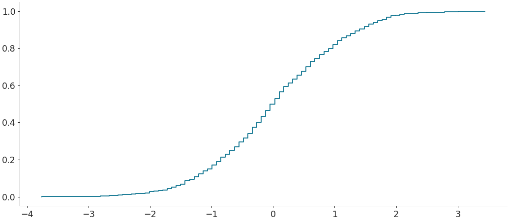
Plot ecdf plot for a given sample

>>> import arviz as az
>>> from scipy.stats import uniform, binom, norm

>>> sample = norm(0,1).rvs(1000)
>>> az.plot_ecdf(sample)

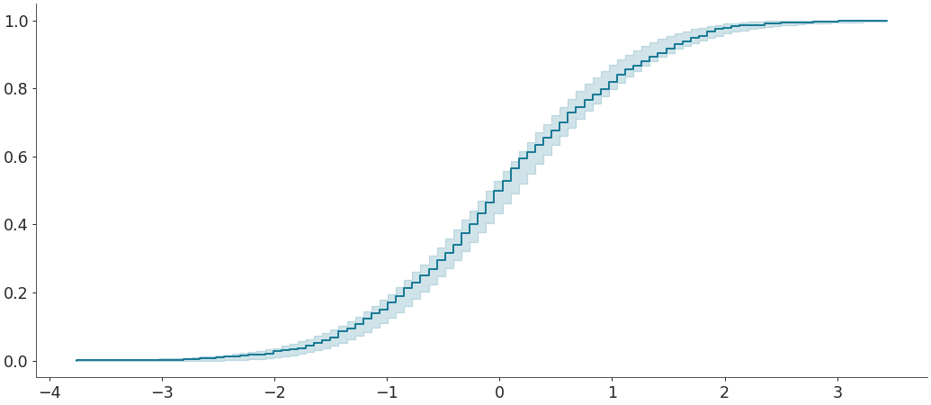
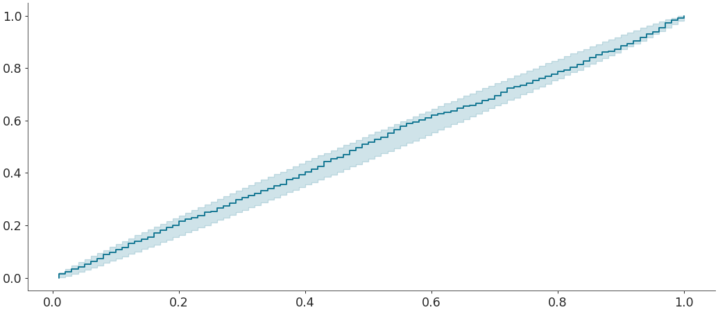
Plot ecdf plot with confidence bands for comparing a given sample w.r.t a given distribution

>>> distribution = norm(0,1)
>>> az.plot_ecdf(sample, cdf = distribution.cdf, confidence_bands = True)

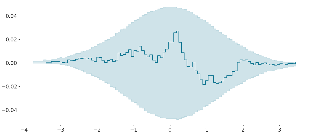
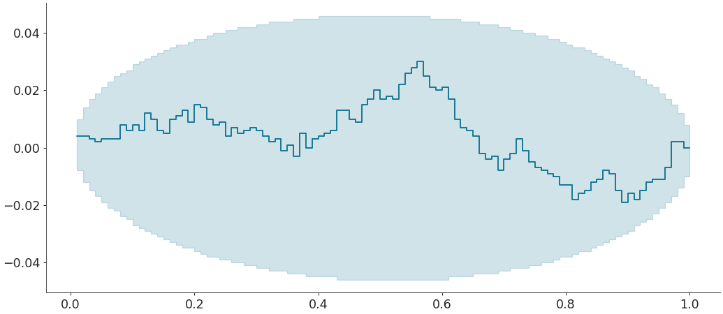
Plot ecdf-difference plot with confidence bands for comparing a given sample w.r.t a given distribution

>>> az.plot_ecdf(sample, cdf = distribution.cdf,
>>>              confidence_bands = True, difference = True)

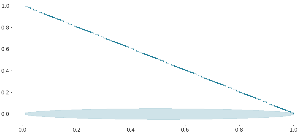
Plot ecdf plot with confidence bands for PIT of sample for comparing a given sample w.r.t a given distribution

>>> az.plot_ecdf(sample, cdf = distribution.cdf,
>>>              confidence_bands = True, pit = True)

Plot ecdf-difference plot with confidence bands for PIT of sample for comparing a given sample w.r.t a given distribution

>>> az.plot_ecdf(sample, cdf = distribution.cdf,
>>>              confidence_bands = True, difference = True, pit = True)

You could also plot the above w.r.t another sample rather than a given distribution. For eg: Plot ecdf-difference plot with confidence bands for PIT of sample for comparing a given sample w.r.t a given sample

>>> sample2 = norm(0,1).rvs(5000)
>>> az.plot_ecdf(sample, sample2, confidence_bands = True, difference = True, pit = True)