arviz.plot_ess#

arviz.plot_ess(idata, var_names=None, filter_vars=None, kind='local', relative=False, coords=None, figsize=None, grid=None, textsize=None, rug=False, rug_kind='diverging', n_points=20, extra_methods=False, min_ess=400, labeller=None, ax=None, extra_kwargs=None, text_kwargs=None, hline_kwargs=None, rug_kwargs=None, backend=None, backend_kwargs=None, show=None, **kwargs)[source]#

Plot quantile, local or evolution of effective sample sizes (ESS).

Parameters

idata: obj: Any object that can be converted to an arviz.InferenceData object Refer to documentation of arviz.convert_to_dataset() for details
var_names: list of variable names, optional: Variables to be plotted. Prefix the variables by ~ when you want to exclude them from the plot.
filter_vars: {None, “like”, “regex”}, optional, default=None: If None (default), interpret var_names as the real variables names. If “like”, interpret var_names as substrings of the real variables names. If “regex”, interpret var_names as regular expressions on the real variables names. A la pandas.filter.
kind: str, optional: Options: local, quantile or evolution, specify the kind of plot.
relative: bool: Show relative ess in plot ress = ess / N.
coords: dict, optional: Coordinates of var_names to be plotted. Passed to xarray.Dataset.sel().
gridtuple: Number of rows and columns. Defaults to None, the rows and columns are automatically inferred.
figsize: tuple, optional: Figure size. If None it will be defined automatically.
textsize: float, optional: Text size scaling factor for labels, titles and lines. If None it will be autoscaled based on figsize.
rug: bool: Plot rug plot of values diverging or that reached the max tree depth.
rug_kind: bool: Variable in sample stats to use as rug mask. Must be a boolean variable.
n_points: int: Number of points for which to plot their quantile/local ess or number of subsets in the evolution plot.
extra_methods: bool, optional: Plot mean and sd ESS as horizontal lines. Not taken into account in evolution kind
min_ess: int: Minimum number of ESS desired. If relative=True the line is plotted at min_ess / n_samples for local and quantile kinds and as a curve following the min_ess / n dependency in evolution kind.
labellerlabeller instance, optional: Class providing the method make_label_vert to generate the labels in the plot titles. Read the Label guide for more details and usage examples.
ax: numpy array-like of matplotlib axes or bokeh figures, optional: A 2D array of locations into which to plot the densities. If not supplied, Arviz will create its own array of plot areas (and return it).
extra_kwargs: dict, optional: If evolution plot, extra_kwargs is used to plot ess tail and differentiate it from ess bulk. Otherwise, passed to extra methods lines.
text_kwargs: dict, optional: Only taken into account when extra_methods=True. kwargs passed to ax.annotate for extra methods lines labels. It accepts the additional key x to set xy=(text_kwargs["x"], mcse)
hline_kwargs: dict, optional: kwargs passed to axhline() or to Span depending on the backend for the horizontal minimum ESS line. For relative ess evolution plots the kwargs are passed to plot() or to line
rug_kwargs: dict: kwargs passed to rug plot.
backend: str, optional: Select plotting backend {“matplotlib”,”bokeh”}. Default “matplotlib”.
backend_kwargs: bool, optional: These are kwargs specific to the backend being used, passed to matplotlib.pyplot.subplots() or bokeh.plotting.figure(). For additional documentation check the plotting method of the backend.
show: bool, optional: Call backend show function.
**kwargs: Passed as-is to matplotlib.axes.Axes.hist() or matplotlib.axes.Axes.plot() function depending on the value of kind.

Returns

axes: matplotlib axes or bokeh figures

See also

ess: Calculate estimate of the effective sample size.

References

Vehtari et al. (2019) see https://arxiv.org/abs/1903.08008

Examples

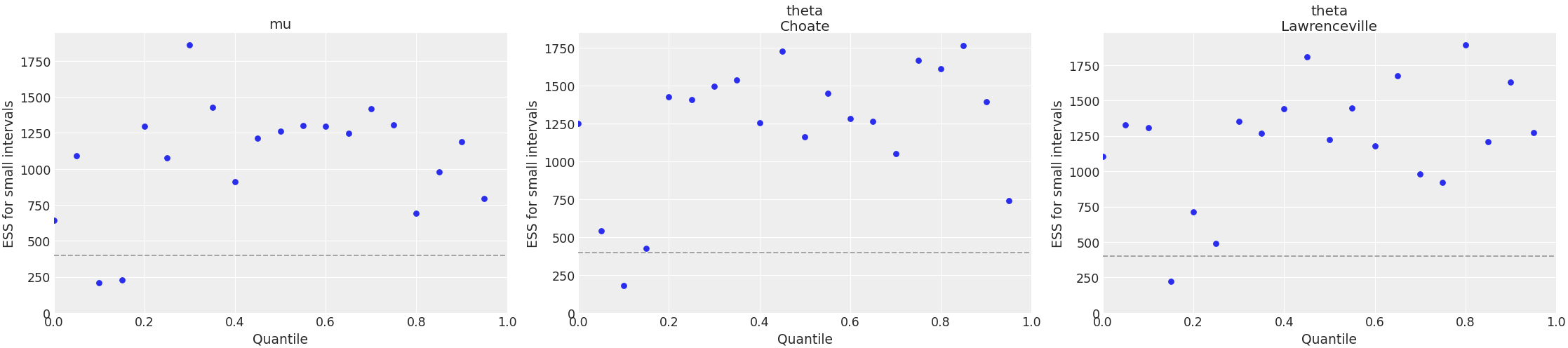
Plot local ESS. This plot, together with the quantile ESS plot, is recommended to check that there are enough samples for all the explored regions of parameter space. Checking local and quantile ESS is particularly relevant when working with HDI intervals as opposed to ESS bulk, which is relevant for point estimates.

>>> import arviz as az
>>> idata = az.load_arviz_data("centered_eight")
>>> coords = {"school": ["Choate", "Lawrenceville"]}
>>> az.plot_ess(
...     idata, kind="local", var_names=["mu", "theta"], coords=coords
... )

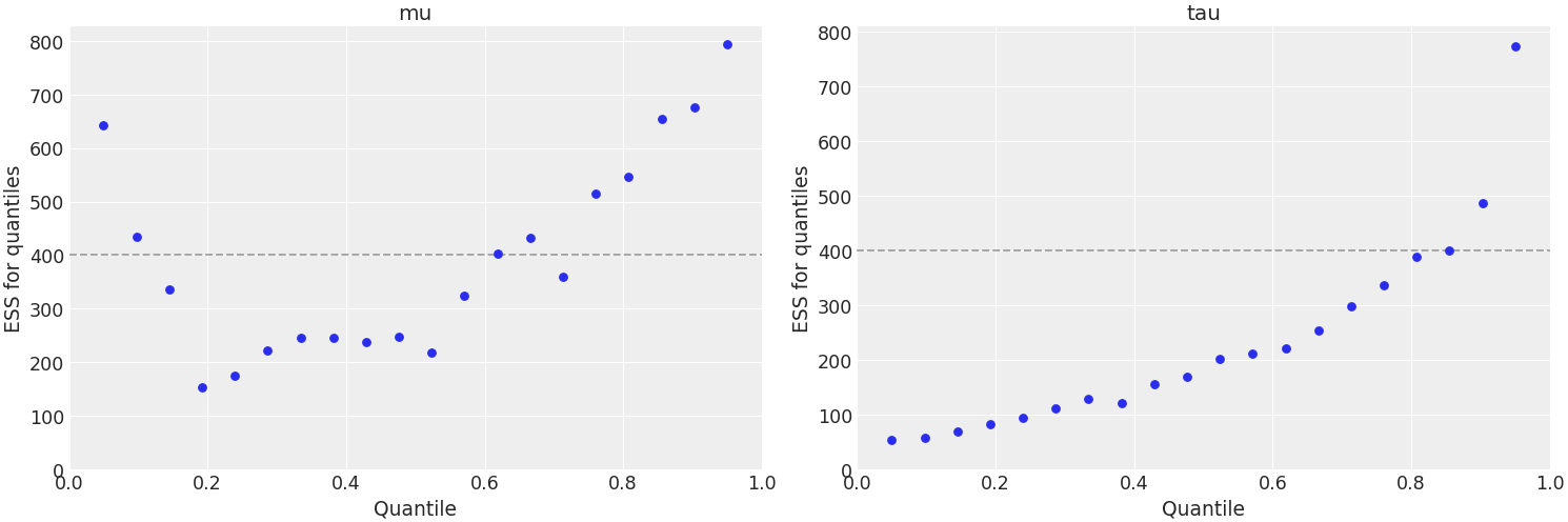
Plot quantile ESS and exclude variables with partial naming

>>> az.plot_ess(
...     idata, kind="quantile", var_names=['~thet'], filter_vars="like", coords=coords
... )

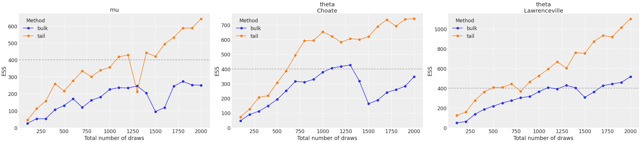
Plot ESS evolution as the number of samples increase. When the model is converging properly, both lines in this plot should be roughly linear.

>>> az.plot_ess(
...     idata, kind="evolution", var_names=["mu", "theta"], coords=coords
... )

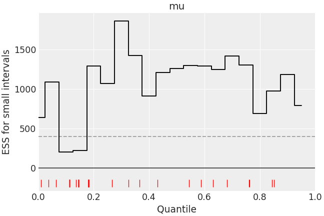
Customize local ESS plot to look like reference paper.

>>> az.plot_ess(
...     idata, kind="local", var_names=["mu"], drawstyle="steps-mid", color="k",
...     linestyle="-", marker=None, rug=True, rug_kwargs={"color": "r"}
... )

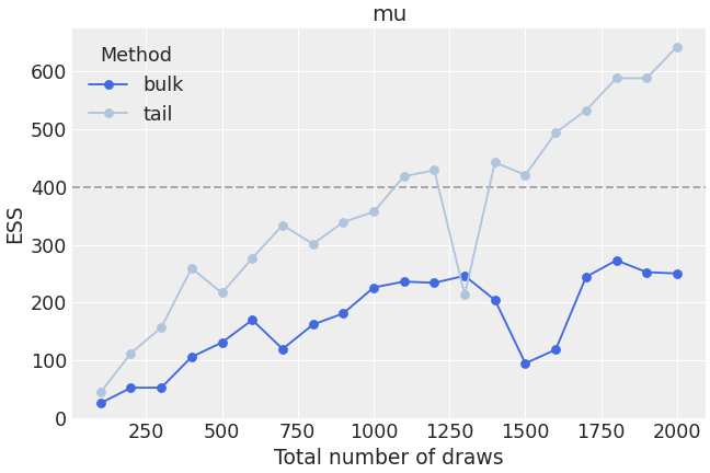
Customize ESS evolution plot to look like reference paper.

>>> extra_kwargs = {"color": "lightsteelblue"}
>>> az.plot_ess(
...     idata, kind="evolution", var_names=["mu"],
...     color="royalblue", extra_kwargs=extra_kwargs
... )

arviz.plot_energy

arviz.plot_forest