arviz.plot_dist#
- arviz.plot_dist(values, values2=None, color='C0', kind='auto', cumulative=False, label=None, rotated=False, rug=False, bw='default', quantiles=None, contour=True, fill_last=True, figsize=None, textsize=None, plot_kwargs=None, fill_kwargs=None, rug_kwargs=None, contour_kwargs=None, contourf_kwargs=None, pcolormesh_kwargs=None, hist_kwargs=None, is_circular=False, ax=None, backend=None, backend_kwargs=None, show=None, **kwargs)[source]#
Plot distribution as histogram or kernel density estimates.
By default continuous variables are plotted using KDEs and discrete ones using histograms
- Parameters
- valuesarray-like
Values to plot.
- values2array-like, optional
Values to plot. If present, a 2D KDE or a hexbin will be estimated.
- colorstring
valid matplotlib color.
- kindstring
By default (“auto”) continuous variables will use the kind defined by rcParam
plot.density_kindand discrete ones will use histograms. To override this use “hist” to plot histograms and “kde” for KDEs.- cumulativebool
If true plot the estimated cumulative distribution function. Defaults to False. Ignored for 2D KDE.
- labelstring
Text to include as part of the legend.
- rotatedbool
Whether to rotate the 1D KDE plot 90 degrees.
- rugbool
If True adds a rugplot. Defaults to False. Ignored for 2D KDE.
- bw: Optional[float or str]
If numeric, indicates the bandwidth and must be positive. If str, indicates the method to estimate the bandwidth and must be one of “scott”, “silverman”, “isj” or “experimental” when
is_circularis False and “taylor” (for now) whenis_circularis True. Defaults to “default” which means “experimental” when variable is not circular and “taylor” when it is.- quantileslist
Quantiles in ascending order used to segment the KDE. Use [.25, .5, .75] for quartiles. Defaults to None.
- contourbool
If True plot the 2D KDE using contours, otherwise plot a smooth 2D KDE. Defaults to True.
- fill_lastbool
If True fill the last contour of the 2D KDE plot. Defaults to True.
- figsizetuple
Figure size. If None it will be defined automatically.
- textsize: float
Text size scaling factor for labels, titles and lines. If None it will be autoscaled based on
figsize. Not implemented for bokeh backend.- plot_kwargsdict
Keywords passed to the pdf line of a 1D KDE. Passed to
arviz.plot_kde()asplot_kwargs.- fill_kwargsdict
Keywords passed to the fill under the line (use fill_kwargs={‘alpha’: 0} to disable fill). Ignored for 2D KDE. Passed to
arviz.plot_kde()asfill_kwargs.- rug_kwargsdict
Keywords passed to the rug plot. Ignored if rug=False or for 2D KDE Use
spacekeyword (float) to control the position of the rugplot. The larger this number the lower the rugplot. Passed toarviz.plot_kde()asrug_kwargs.- contour_kwargsdict
Keywords passed to the contourplot. Ignored for 1D KDE.
- contourf_kwargsdict
Keywords passed to
matplotlib.axes.Axes.contourf(). Ignored for 1D KDE.- pcolormesh_kwargsdict
Keywords passed to
matplotlib.axes.Axes.pcolormesh(). Ignored for 1D KDE.- hist_kwargsdict
Keyword arguments used to customize the histogram. Ignored when plotting a KDE. They are passed to
matplotlib.axes.Axes.hist()if using matplotlib, or tobokeh.plotting.Figure.quad()if using bokeh. In bokeh case, the following extra keywords are also supported:color: replaces thefill_colorandline_colorof thequadmethodbins: taken fromhist_kwargsand passed tonumpy.histogram()insteaddensity: normalize histogram to represent a probability density function, Defaults toTruecumulative: plot the cumulative counts. Defaults toFalse
- is_circular{False, True, “radians”, “degrees”}. Default False.
Select input type {“radians”, “degrees”} for circular histogram or KDE plot. If True, default input type is “radians”. When this argument is present, it interprets the values passed are from a circular variable measured in radians and a circular KDE is used. Inputs in “degrees” will undergo an internal conversion to radians. Only valid for 1D KDE. Defaults to False.
- ax: axes, optional
Matplotlib axes or bokeh figures.
- backend: str, optional
Select plotting backend {“matplotlib”,”bokeh”}. Default “matplotlib”.
- backend_kwargs: bool, optional
These are kwargs specific to the backend being used, passed to
matplotlib.pyplot.subplots()orbokeh.plotting.figure(). For additional documentation check the plotting method of the backend.- showbool, optional
Call backend show function.
- Returns
- axesmatplotlib axes or bokeh figures
See also
plot_posteriorPlot Posterior densities in the style of John K. Kruschke’s book.
plot_densityGenerate KDE plots for continuous variables and histograms for discrete ones.
plot_kde1D or 2D KDE plot taking into account boundary conditions.
Examples
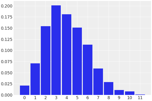
Plot an integer distribution
>>> import numpy as np
>>> import arviz as az
>>> a = np.random.poisson(4, 1000)
>>> az.plot_dist(a)
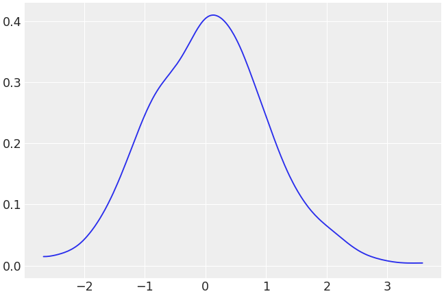
Plot a continuous distribution
>>> b = np.random.normal(0, 1, 1000)
>>> az.plot_dist(b)
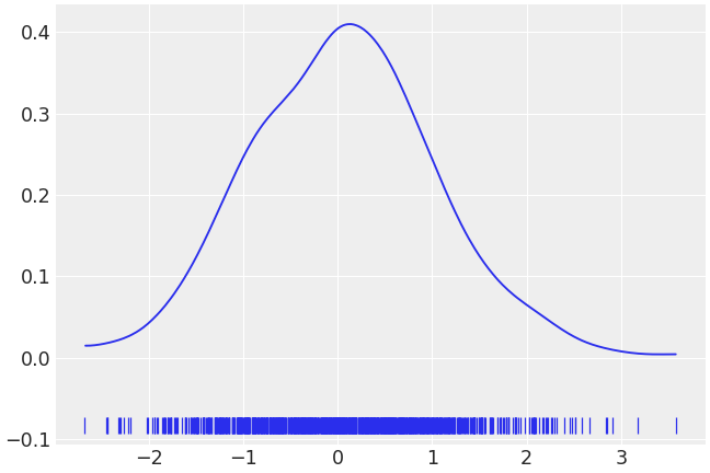
Add a rug under the Gaussian distribution
>>> az.plot_dist(b, rug=True)
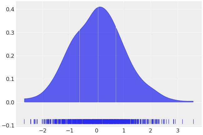
Segment into quantiles
>>> az.plot_dist(b, rug=True, quantiles=[.25, .5, .75])
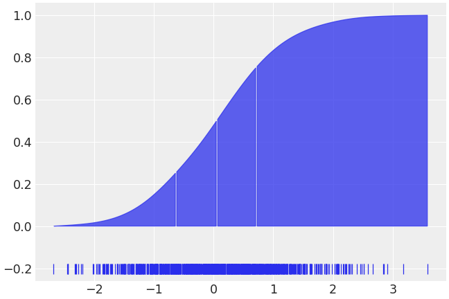
Plot as the cumulative distribution
>>> az.plot_dist(b, rug=True, quantiles=[.25, .5, .75], cumulative=True)