arviz.plot_violin¶

arviz.plot_violin(data, var_names=None, filter_vars=None, transform=None, quartiles=True, rug=False, hdi_prob=None, shade=0.35, bw='default', circular=False, sharex=True, sharey=True, grid=None, figsize=None, textsize=None, labeller=None, ax=None, shade_kwargs=None, rug_kwargs=None, backend=None, backend_kwargs=None, show=None)[source]¶

Plot posterior of traces as violin plot.

Parameters

data: obj: Any object that can be converted to an az.InferenceData object Refer to documentation of az.convert_to_dataset for details
var_names: list of variable names, optional: Variables to be plotted, if None all variable are plotted. Prefix the variables by ~ when you want to exclude them from the plot.
filter_vars: {None, “like”, “regex”}, optional, default=None: If None (default), interpret var_names as the real variables names. If “like”, interpret var_names as substrings of the real variables names. If “regex”, interpret var_names as regular expressions on the real variables names. A la pandas.filter.
transform: callable: Function to transform data (defaults to None i.e. the identity function)
quartiles: bool, optional: Flag for plotting the interquartile range, in addition to the hdi_prob*100% intervals. Defaults to True
rug: bool: If True adds a jittered rugplot. Defaults to False.
hdi_prob: float, optional: Plots highest posterior density interval for chosen percentage of density. Defaults to 0.94.
shade: float: Alpha blending value for the shaded area under the curve, between 0 (no shade) and 1 (opaque). Defaults to 0
bw: float or str, optional: If numeric, indicates the bandwidth and must be positive. If str, indicates the method to estimate the bandwidth and must be one of “scott”, “silverman”, “isj” or “experimental” when circular is False and “taylor” (for now) when circular is True. Defaults to “default” which means “experimental” when variable is not circular and “taylor” when it is.
circular: bool, optional.: If True, it interprets values is a circular variable measured in radians and a circular KDE is used. Defaults to False.
gridtuple: Number of rows and columns. Defaults to None, the rows and columns are automatically inferred.
figsize: tuple: Figure size. If None it will be defined automatically.
textsize: int: Text size of the point_estimates, axis ticks, and highest density interval. If None it will be autoscaled based on figsize.
labellerlabeller instance, optional: Class providing the method make_label_vert to generate the labels in the plot titles. Read the Label guide for more details and usage examples.
sharex: bool: Defaults to True, violinplots share a common x-axis scale.
sharey: bool: Defaults to True, violinplots share a common y-axis scale.
ax: numpy array-like of matplotlib axes or bokeh figures, optional: A 2D array of locations into which to plot the densities. If not supplied, Arviz will create its own array of plot areas (and return it).
shade_kwargs: dicts, optional: Additional keywords passed to fill_between, or barh to control the shade.
rug_kwargs: dict: Keywords passed to the rug plot. If true only the righ half side of the violin will be plotted.
backend: str, optional: Select plotting backend {“matplotlib”,”bokeh”}. Default “matplotlib”.
backend_kwargs: bool, optional: These are kwargs specific to the backend being used. For additional documentation check the plotting method of the backend.
show: bool, optional: Call backend show function.

Returns

axes: matplotlib axes or bokeh figures

Notes

If multiple chains are provided for a variable they will be combined

Examples

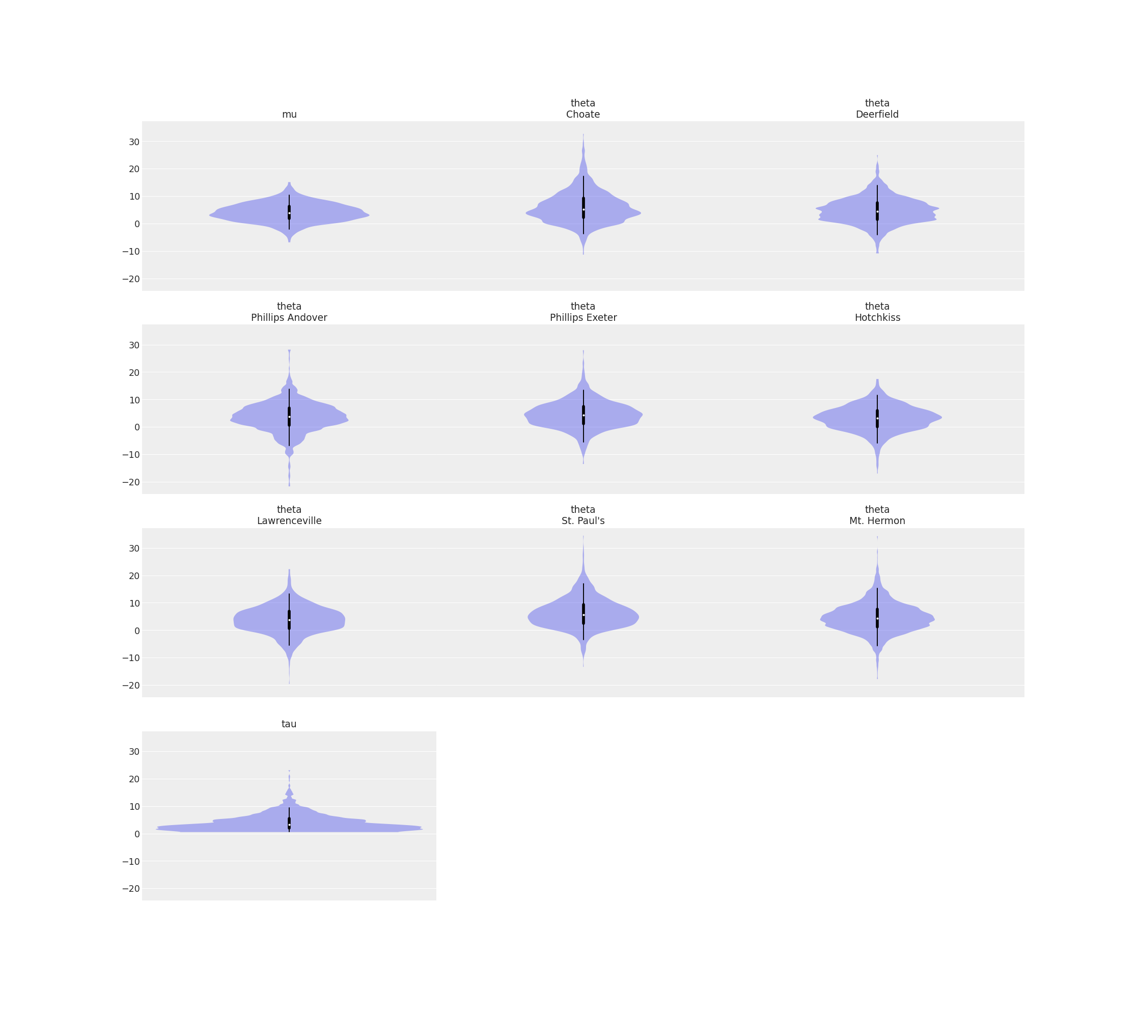
Show a default violin plot

>>> import arviz as az
>>> data = az.load_arviz_data('centered_eight')
>>> az.plot_violin(data)

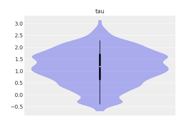
Show a default violin plot, but with a transformation applied to the data

>>> az.plot_violin(data, var_names="tau", transform=np.log)

arviz.plot_ts

Stats