arviz.plot_lm
-
arviz.plot_lm(y, idata=None, x=None, y_model=None, y_hat=None, num_samples=50, kind_pp='samples', kind_model='lines', xjitter=False, plot_dim=None, backend=None, y_kwargs=None, y_hat_plot_kwargs=None, y_hat_fill_kwargs=None, y_model_plot_kwargs=None, y_model_fill_kwargs=None, backend_kwargs=None, show=None, figsize=None, textsize=None, axes=None, legend=True, grid=True)[source]¶ Posterior predictive and mean plots for regression-like data.
- Parameters
- ystr or DataArray or ndarray
If str, variable name from observed_data
- idataInferenceData, Optional
Optional only if y is not str
- xstr, tuple of strings, DataArray or array-like, optional
If str or tuple, variable name from constant_data If ndarray, could be 1D, or 2D for multiple plots If none, coords name of y (y should be DataArray).
- y_modelstr or Sequence, Optional
If str, variable name from posterior. Its dimensions should be same as y plus added chains and draws.
- y_hatstr, Optional
If str, variable name from posterior_predictive. Its dimensions should be same as y plus added chains and draws.
- num_samplesint, Optional, Default 50
Significant if kind_pp is “samples” or kind_model is “lines”. Number of samples to be drawn from posterior predictive or
- kind_pp{“samples”, “hdi”}, Default “samples”
Options to visualize uncertainty in data.
- kind_model{“lines”, “hdi”}, Default “lines”
Options to visualize uncertainty in mean of the data.
- plot_dimstr, Optional
Necessary if y is multidimensional.
- backendstr, Optional
Select plotting backend {“matplotlib”,”bokeh”}. Default “matplotlib”.
- y_kwargsdict, optional
Passed to
matplotlib.axes.Axes.plot()in matplotlib andbokeh.plotting.Figure.circle()in bokeh- y_hat_plot_kwargsdict, optional
Passed to
matplotlib.axes.Axes.plot()in matplotlib andbokeh.plotting.Figure.circle()in bokeh- y_hat_fill_kwargsdict, optional
Passed to {func}`~arviz.plot_hdi`
- y_model_plot_kwargsdict, optional
Passed to
matplotlib.axes.Axes.plot()in matplotlib andbokeh.plotting.Figure.line()in bokeh- y_model_fill_kwargsdict, optional
Significant if kind_model is “hdi”. Passed to
plot_hdi()- backend_kwargsdict, optional
These are kwargs specific to the backend being used. Passed to :meth: mpl:matplotlib.pyplot.subplots or :meth: bokeh:bokeh.plotting.figure
- figsizetuple, optional
Figure size. If None it will be defined automatically.
- textsizefloat, optional
Text size scaling factor for labels, titles and lines. If None it will be autoscaled based on figsize.
- axesnumpy array-like of matplotlib axes or bokeh figures, optional
A 2D array of locations into which to plot the densities. If not supplied, Arviz will create its own array of plot areas (and return it).
- show: bool, optional
Call backend show function.
- legendbool, optional
Add legend to figure. By default True.
- gridbool, optional
Add grid to figure. By default True.
- Returns
- axes: matplotlib axes or bokeh figures
Examples
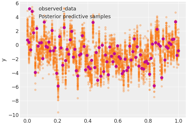
Plot regression default plot
>>> import arviz as az
>>> import numpy as np
>>> import xarray as xr
>>> idata = az.load_arviz_data('regression1d')
>>> x = xr.DataArray(np.linspace(0, 1, 100))
>>> idata.posterior["y_model"] = idata.posterior["intercept"] + idata.posterior["slope"]*x
>>> az.plot_lm(idata=idata, y="y", x=x)
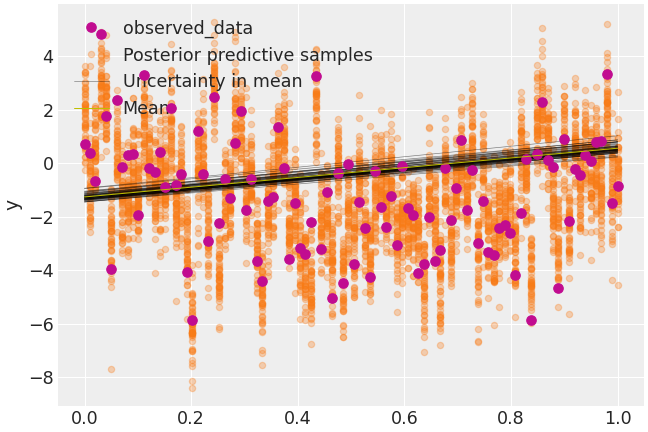
Plot regression data and mean uncertainty
>>> az.plot_lm(idata=idata, y="y", x=x, y_model="y_model")
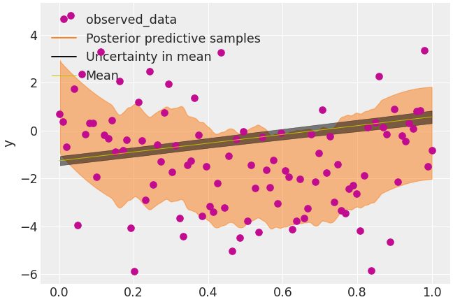
Plot regression data and mean uncertainty in hdi form
>>> az.plot_lm(
...     idata=idata, y="y", x=x, y_model="y_model", kind_pp="hdi", kind_model="hdi"
... )
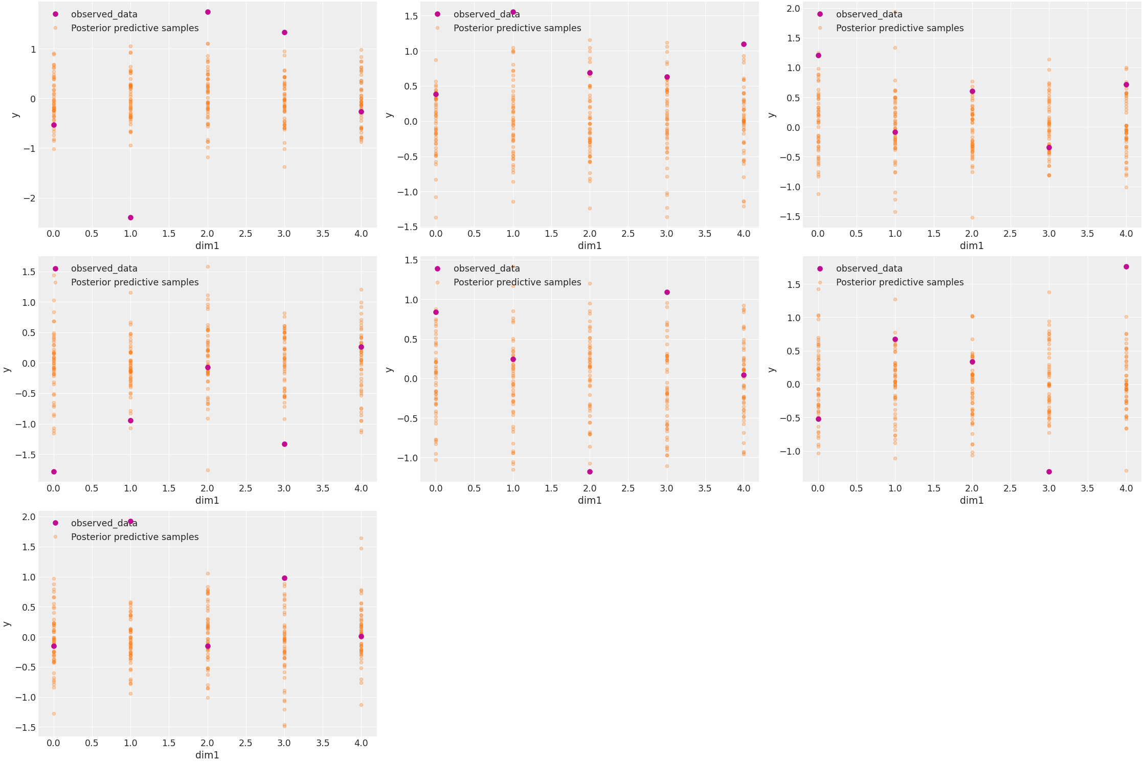
Plot regression data for multi-dimensional y using plot_dim
>>> data = az.from_dict(
...     observed_data = { "y": np.random.normal(size=(5, 7)) },
...     posterior_predictive = {"y": np.random.randn(4, 1000, 5, 7) / 2},
...     dims={"y": ["dim1", "dim2"]},
...     coords={"dim1": range(5), "dim2": range(7)}
... )
>>> az.plot_lm(idata=data, y="y", plot_dim="dim1")