arviz.plot_joint
-
arviz.plot_joint(data, group='posterior', var_names=None, filter_vars=None, transform=None, coords=None, figsize=None, textsize=None, kind='scatter', gridsize='auto', contour=True, fill_last=True, joint_kwargs=None, marginal_kwargs=None, ax=None, backend=None, backend_kwargs=None, show=None)[source]¶ Plot a scatter or hexbin of two variables with their respective marginals distributions.
- Parameters
- data: obj
Any object that can be converted to an az.InferenceData object Refer to documentation of az.convert_to_dataset for details
- group: str, optional
Specifies which InferenceData group should be plotted. Defaults to ‘posterior’.
- var_names: str or iterable of str
Variables to be plotted. Iterable of two variables or one variable (with subset having exactly 2 dimensions) are required. Prefix the variables by ~ when you want to exclude them from the plot.
- filter_vars: {None, “like”, “regex”}, optional, default=None
If None (default), interpret var_names as the real variables names. If “like”, interpret var_names as substrings of the real variables names. If “regex”, interpret var_names as regular expressions on the real variables names. A la pandas.filter.
- transform: callable
Function to transform data (defaults to None i.e. the identity function)
- coords: mapping, optional
Coordinates of var_names to be plotted. Passed to Dataset.sel
- figsize: tuple
Figure size. If None it will be defined automatically.
- textsize: float
Text size scaling factor for labels, titles and lines. If None it will be autoscaled based on figsize.
- kind: str
Type of plot to display (scatter, kde or hexbin)
- gridsize: int or (int, int), optional.
The number of hexagons in the x-direction. Ignored when hexbin is False. See plt.hexbin for details
- contour: bool
If True plot the 2D KDE using contours, otherwise plot a smooth 2D KDE. Defaults to True.
- fill_last: bool
If True fill the last contour of the 2D KDE plot. Defaults to True.
- joint_kwargs: dicts, optional
Additional keywords modifying the join distribution (central subplot)
- marginal_kwargs: dicts, optional
Additional keywords modifying the marginals distributions (top and right subplot)
- ax: tuple of axes, optional
Tuple containing (ax_joint, ax_hist_x, ax_hist_y). If None, a new figure and axes will be created. Matplotlib axes or bokeh figures.
- backend: str, optional
Select plotting backend {“matplotlib”,”bokeh”}. Default “matplotlib”.
- backend_kwargs: bool, optional
These are kwargs specific to the backend being used. For additional documentation check the plotting method of the backend.
- show: bool, optional
Call backend show function.
- Returns
- axes: matplotlib axes or bokeh figures
ax_joint: joint (central) distribution ax_hist_x: x (top) distribution ax_hist_y: y (right) distribution
Examples
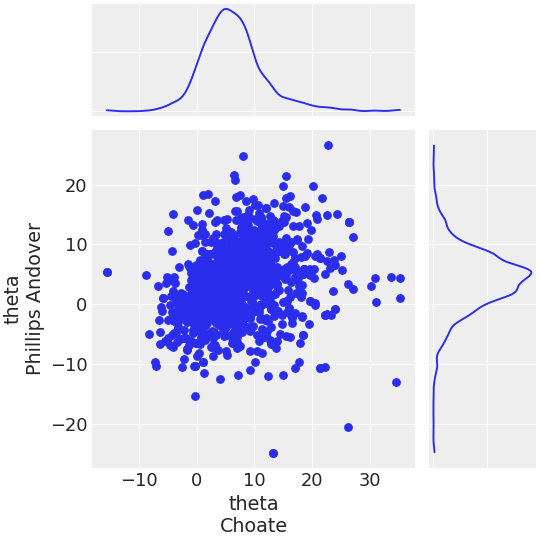
Scatter Joint plot
>>> import arviz as az
>>> data = az.load_arviz_data('non_centered_eight')
>>> az.plot_joint(data,
>>>             var_names=['theta'],
>>>             coords={'school': ['Choate', 'Phillips Andover']},
>>>             kind='scatter',
>>>             figsize=(6, 6))
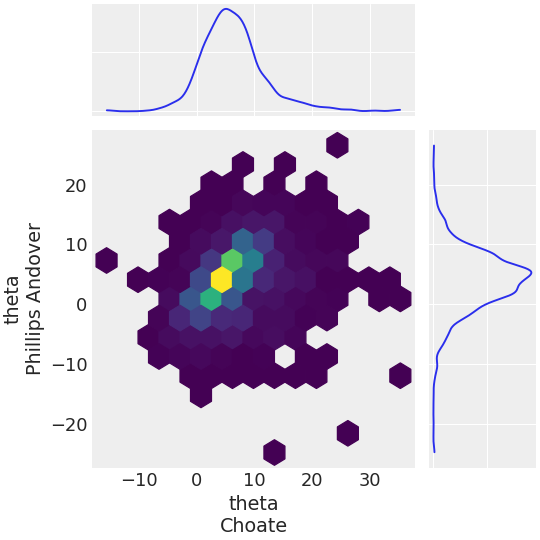
Hexbin Joint plot
>>> az.plot_joint(data,
>>>             var_names=['theta'],
>>>             coords={'school': ['Choate', 'Phillips Andover']},
>>>             kind='hexbin',
>>>             figsize=(6, 6))
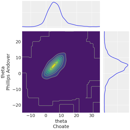
KDE Joint plot
>>> az.plot_joint(data,
>>>                 var_names=['theta'],
>>>                 coords={'school': ['Choate', 'Phillips Andover']},
>>>                 kind='kde',
>>>                 figsize=(6, 6))
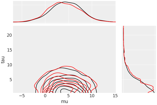
Overlaid plots:
>>> data2 = az.load_arviz_data("centered_eight")
>>> kde_kwargs = {"contourf_kwargs": {"alpha": 0}, "contour_kwargs": {"colors": "k"}}
>>> ax = az.plot_joint(
...     data, var_names=("mu", "tau"), kind="kde", fill_last=False,
...     joint_kwargs=kde_kwargs, marginal_kwargs={"color": "k"}
... )
>>> kde_kwargs["contour_kwargs"]["colors"] = "r"
>>> az.plot_joint(
...     data2, var_names=("mu", "tau"), kind="kde", fill_last=False,
...     joint_kwargs=kde_kwargs, marginal_kwargs={"color": "r"}, ax=ax
... )