arviz.plot_ts¶

arviz.plot_ts(idata, y, x=None, y_hat=None, y_holdout=None, y_forecasts=None, x_holdout=None, plot_dim=None, holdout_dim=None, num_samples=100, backend=None, backend_kwargs=None, y_kwargs=None, y_hat_plot_kwargs=None, y_mean_plot_kwargs=None, vline_kwargs=None, textsize=None, figsize=None, legend=True, axes=None, show=None)[source]¶

Plot timeseries data.

Parameters

idataInferenceData: InferenceData object.
ystr: Variable name from observed_data. Values to be plotted on y-axis before holdout.
xstr, Optional: Values to be plotted on x-axis before holdout. If none, coords of y dims is chosen.
y_hatstr, optional: Variable name from posterior_predictive. Assumed to be of shape (chain, draw, *y_dims).
y_holdoutstr, optional: Variable name from observed_data. It represents the observed data after the holdout period. Usefull while testing the model, when you want to compare observed test data with predictions/forecasts.
y_forecastsstr, optional: Variable name from posterior_predictive. It represents forecasts (posterior predictive) values after holdout preriod. Usefull to compare observed vs predictions/forecasts. Assumed shape (chain, draw, *shape).
x_holdoutstr, Defaults to coords of y.: Variable name from constant_data. If None, coords of y_holdout or coords of y_forecast (either of the two available) is chosen.
plot_dim: str, Optional: Should be present in y.dims Necessary for selection of x if x is None and y is multidimensional.
holdout_dim: str, Optional: Should be present in y_holdout.dims or y_forecats.dims. Necessary to choose x_holdout if x is None and if y_holdout or y_forecasts is multidimensional.
num_samplesint, default 100: Number of posterior predictive samples drawn from y_hat and y_forecasts.
backend{“matplotlib”, “bokeh”}, default “matplotlib”: Select plotting backend.
y_kwargsdict, optional: Passed to matplotlib.axes.Axes.plot() in matplotlib.
y_hat_plot_kwargsdict, optional: Passed to matplotlib.axes.Axes.plot() in matplotlib.
y_mean_plot_kwargsdict, optional: Passed to matplotlib.axes.Axes.plot() in matplotlib.
vline_kwargsdict, optional: Passed to matplotlib.axes.Axes.axvline() in matplotlib.
backend_kwargsdict, optional: These are kwargs specific to the backend being used. Passed to :func: mpl:matplotlib.pyplot.subplots.
figsizetuple, optional: Figure size. If None it will be defined automatically.
textsizefloat, optional: Text size scaling factor for labels, titles and lines. If None it will be autoscaled based on figsize.

Returns

axes: matplotlib axes or bokeh figures.

Examples

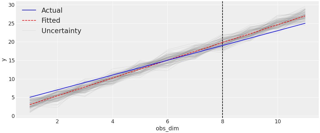
Plot timeseries default plot

>>> import arviz as az
>>> nchains, ndraws = (4, 500)
>>> obs_data = {
...     "y": 2 * np.arange(1, 9) + 3,
...     "z": 2 * np.arange(8, 12) + 3,
... }
>>> posterior_predictive = {
...     "y": np.random.normal(
...         (obs_data["y"] * 1.2) - 3, size=(nchains, ndraws, len(obs_data["y"]))
...     ),
...     "z": np.random.normal(
...         (obs_data["z"] * 1.2) - 3, size=(nchains, ndraws, len(obs_data["z"]))
...     ),
...  }
>>> idata = az.from_dict(
...     observed_data=obs_data,
...     posterior_predictive=posterior_predictive,
...     coords={"obs_dim": np.arange(1, 9), "pred_dim": np.arange(8, 12)},
...     dims={"y": ["obs_dim"], "z": ["pred_dim"]},
... )
>>> ax = az.plot_ts(idata=idata, y="y", y_holdout="z")

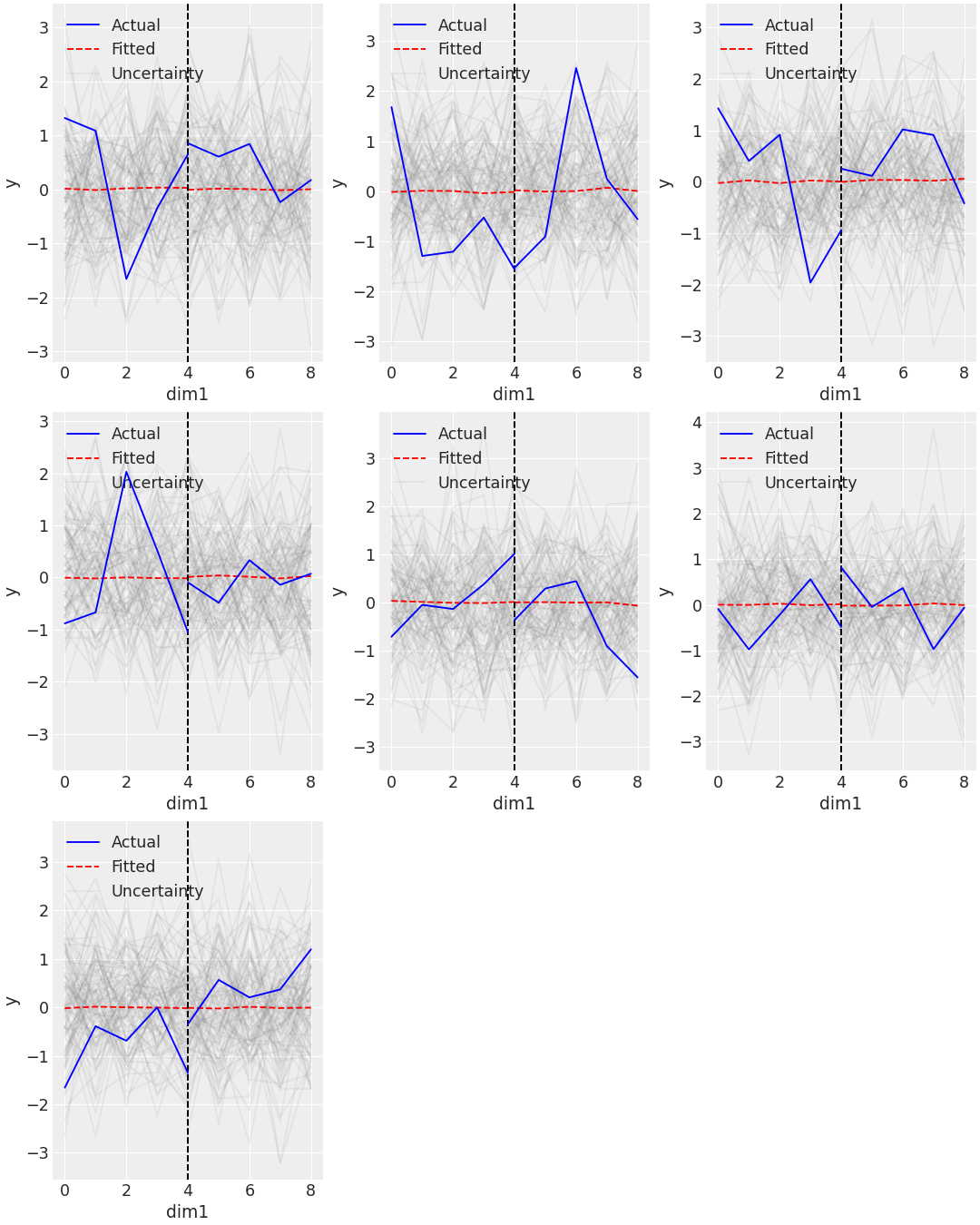
Plot timeseries multidim plot

>>> ndim1, ndim2 = (5, 7)
>>> data = {
...     "y": np.random.normal(size=(ndim1, ndim2)),
...     "z": np.random.normal(size=(ndim1, ndim2)),
... }
>>> posterior_predictive = {
...     "y": np.random.randn(nchains, ndraws, ndim1, ndim2),
...     "z": np.random.randn(nchains, ndraws, ndim1, ndim2),
... }
>>> const_data = {"x": np.arange(1, 6), "x_pred": np.arange(5, 10)}
>>> idata = az.from_dict(
...     observed_data=data,
...     posterior_predictive=posterior_predictive,
...     constant_data=const_data,
...     dims={
...         "y": ["dim1", "dim2"],
...         "z": ["holdout_dim1", "holdout_dim2"],
...     },
...     coords={
...         "dim1": range(ndim1),
...         "dim2": range(ndim2),
...         "holdout_dim1": range(ndim1 - 1, ndim1 + 4),
...         "holdout_dim2": range(ndim2 - 1, ndim2 + 6),
...     },
... )
>>> az.plot_ts(
...     idata=idata,
...     y="y",
...     plot_dim="dim1",
...     y_holdout="z",
...     holdout_dim="holdout_dim1",
... )

arviz.plot_trace

arviz.plot_violin