Plots’ arguments guide#
Arviz plot module is used for plotting data. It consists many functions that each serve different purposes. Most of these plotting functions have common arguments. These common arguments are explained in the following examples, which use one specific function to illustrate the usage but the behaviour described here will be the same for the other functions with the same argument.
This page can be downloaded as a Python script
or as a Jupyter notebook.
import arviz as az
import numpy as np

centered_eight = az.load_arviz_data('centered_eight')
non_centered_eight = az.load_arviz_data('non_centered_eight')

x_data = np.random.normal(0, 1, 100)
y_data = np.random.normal(2 + x_data * 0.5, 0.5, (2, 50, 100))
az.style.use("arviz-darkgrid")
Warning
Page in construction
var_names#
Variables to be plotted. If None all variables are plotted.
Prefix the variables by ~ when you want to exclude them from the plot.
Let’s see the examples.
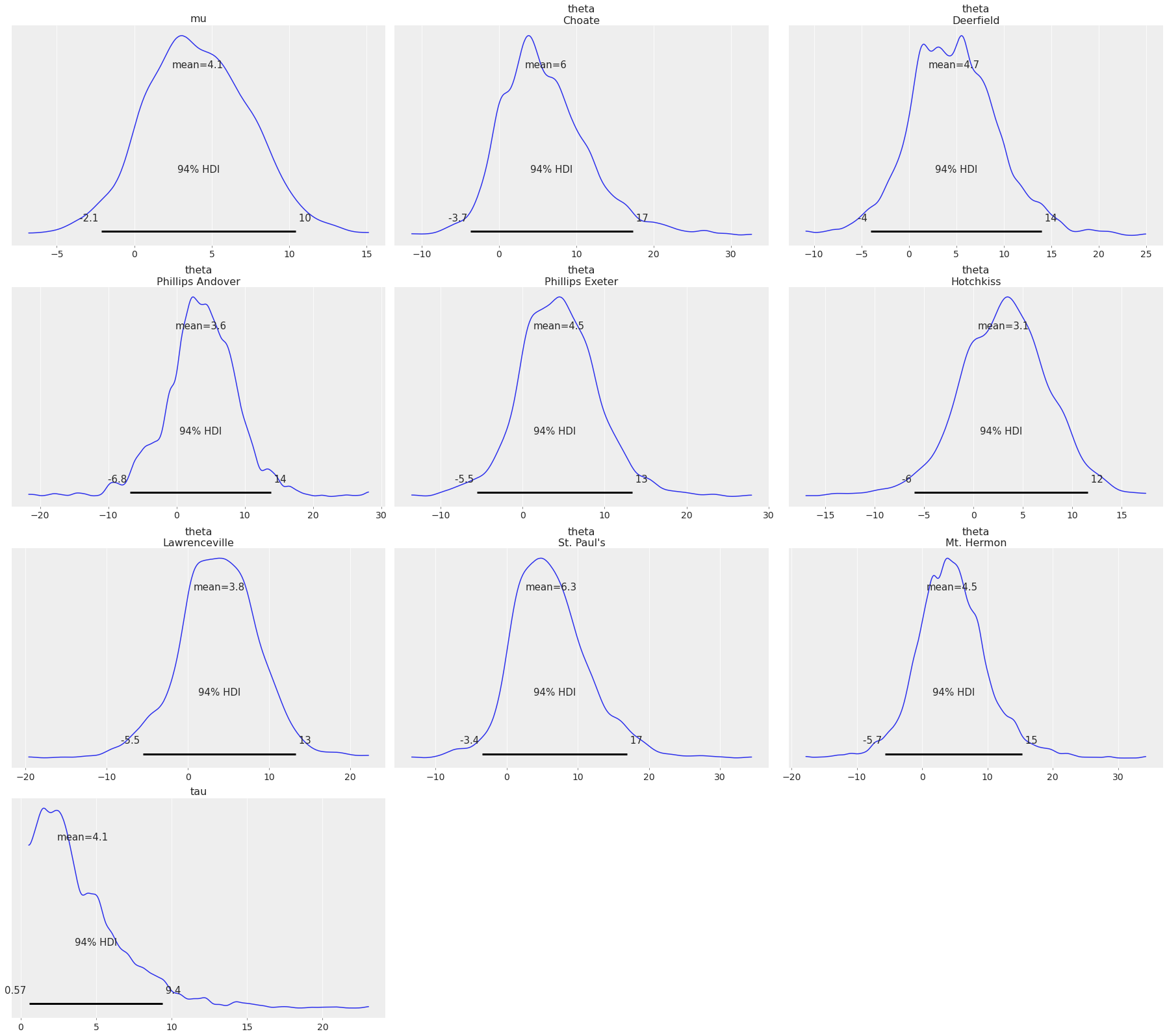
Plot all variables, which is the default behavior:
az.plot_posterior(centered_eight);
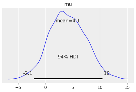
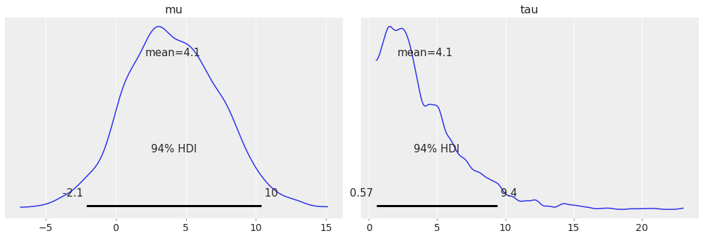
Plot one variable by setting var_names="var1":
az.plot_posterior(centered_eight, var_names='mu');
Plot subset variables by specifying variable name exactly:
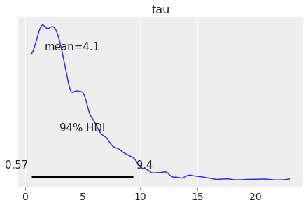
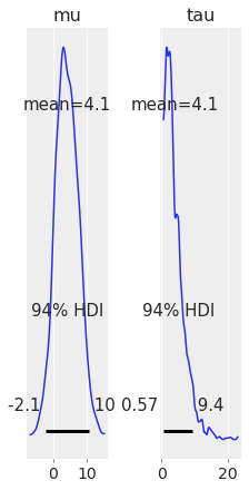
az.plot_posterior(centered_eight, var_names=['mu', 'tau']);
Use var_names to indicate which variables to exclude with the ~ prefix:
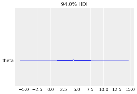
az.plot_posterior(centered_eight, var_names=['~mu', '~theta']);
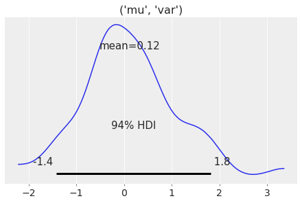
Variables do not need to be strings to be used. Anything that is hashable will work.
mu = ("mu", "var")
samples = np.random.normal(0, 1, 100)
data = az.dict_to_dataset({mu: samples})
az.plot_posterior(data);
filter_vars#
If None (default), interpret var_names as the real variables names,
as shown in the previous section.
This argument is inspired in pandas.DataFrame.filter().
If “like”, interpret var_names as substrings of the real variables names.
Each substring is checked against all present variable names and the
list of matching variables to be plotted is generated.
az.plot_posterior(centered_eight, var_names='ta', filter_vars="like");
Both tau and theta have ta inside them, so only mu is excluded in this case.
You can also use lists and you can also use the ~ prefix to indicate
that all variables containing that substring should be excluded.
az.plot_posterior(centered_eight, var_names='~ta', filter_vars="like");
If “regex”, interpret var_names as regular expressions on the real variables names.
The regular expression u$ matches the letter “u” at the end of the line
(end of the variable name in this case). So it will match mu and tau
variables:
az.plot_posterior(centered_eight, var_names="u$", filter_vars="regex");
Again, like with filter_vars="like", a list of regular expressions can
also be provided as well as negative conditions with ~.
Note
When providing a list of regular expressions and substring matches, they are expanded independently.
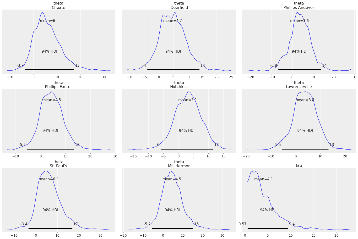
coords#
Dictionary mapping dimensions to selected coordinates to be plotted. Dimensions without a mapping specified will include the data corresponding to all coordinate values for that dimension. It defaults to including all coordinates for all dimensions.
Using coords argument to plot only a subset of data:
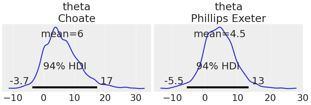
coords = {"school": ["Choate", "Phillips Exeter"]};
az.plot_posterior(centered_eight, var_names=["mu", "theta"], coords=coords);
combined#
Flag for combining multiple chains into a single chain.
When True, chains are combined into a single plot/line,
when False each chain is plotted independently
(either beside each other or each in their own subplot).
While the behaviour of the parameter is the same in all plots,
its default depends on the plotting function.
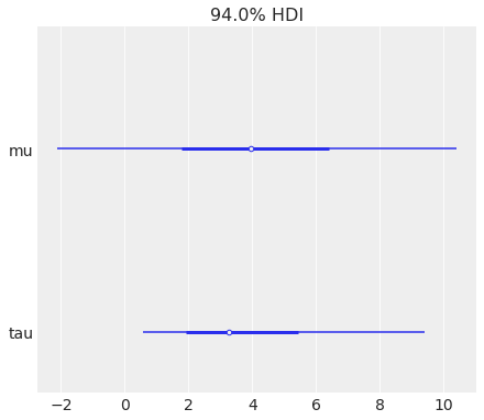
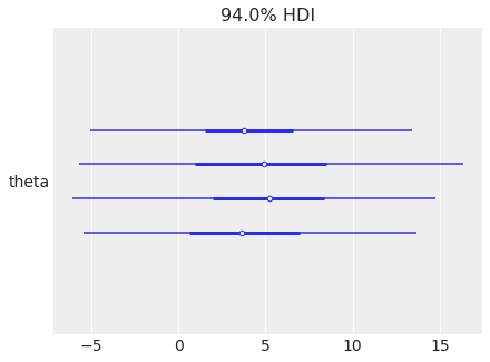
Plot each chain separately:
az.plot_forest(centered_eight, var_names=["mu", "tau"]);
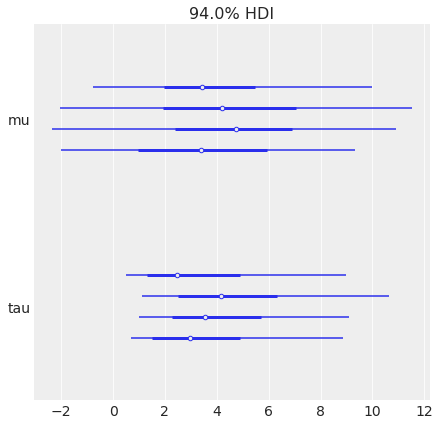
Plot all chains collapsed into a single line:
az.plot_forest(centered_eight, var_names=["mu", "tau"], combined=True);
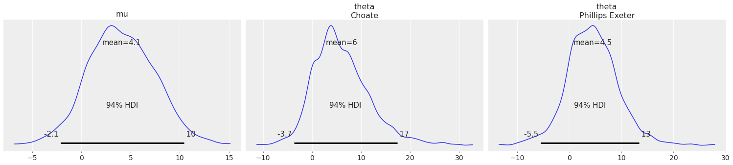
combine_dims#
Set like argument containing dimensions to reduce for plots that represent probability
distributions. When used, the dimensions on combine_dims are added to chain and
draw dimensions and reduced to generate a single KDE/histogram/dot plot from >2D
arrays.
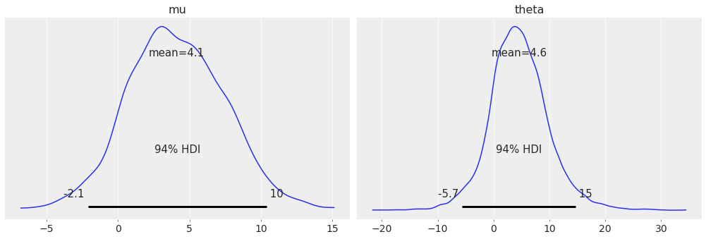
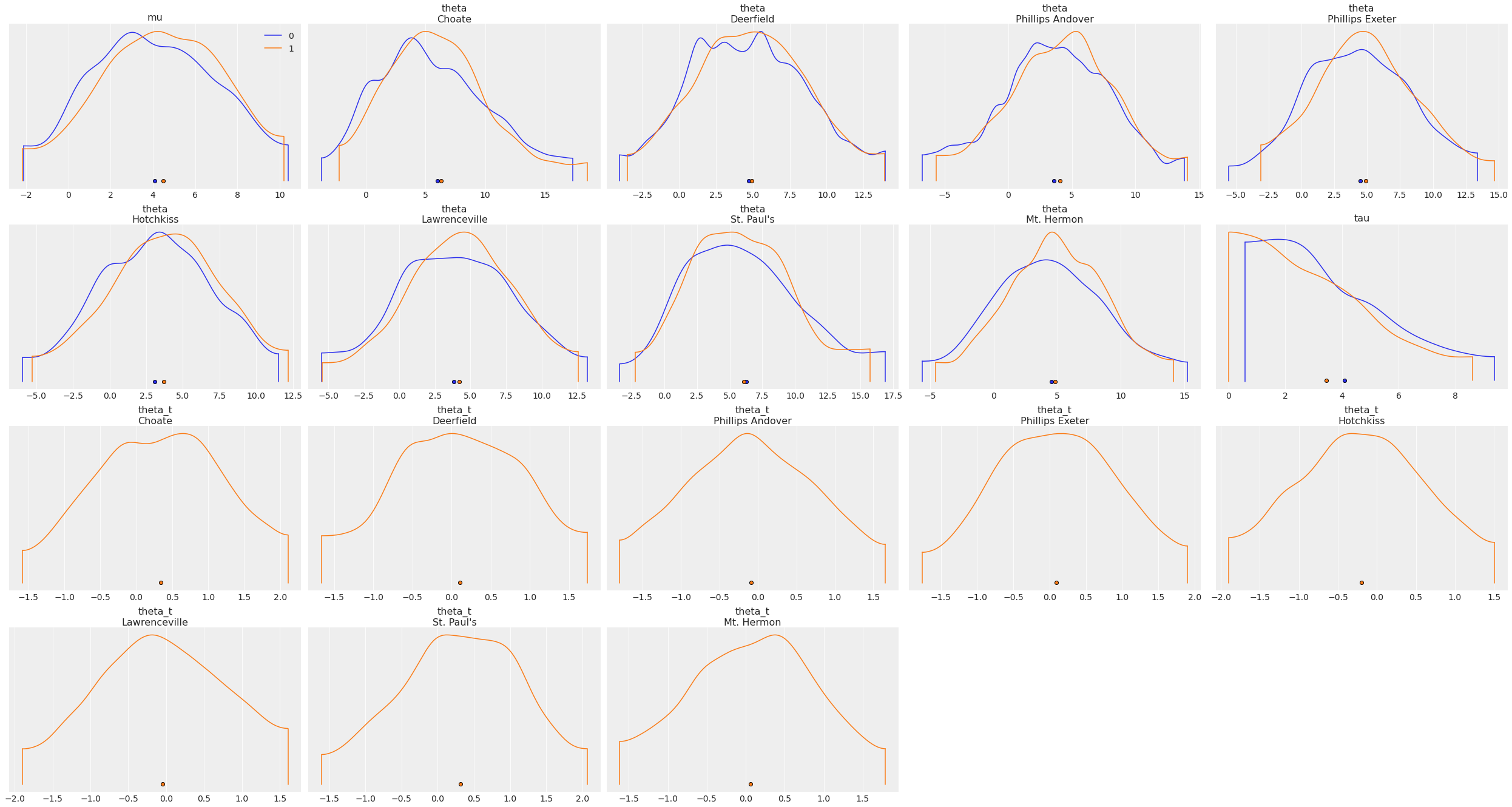
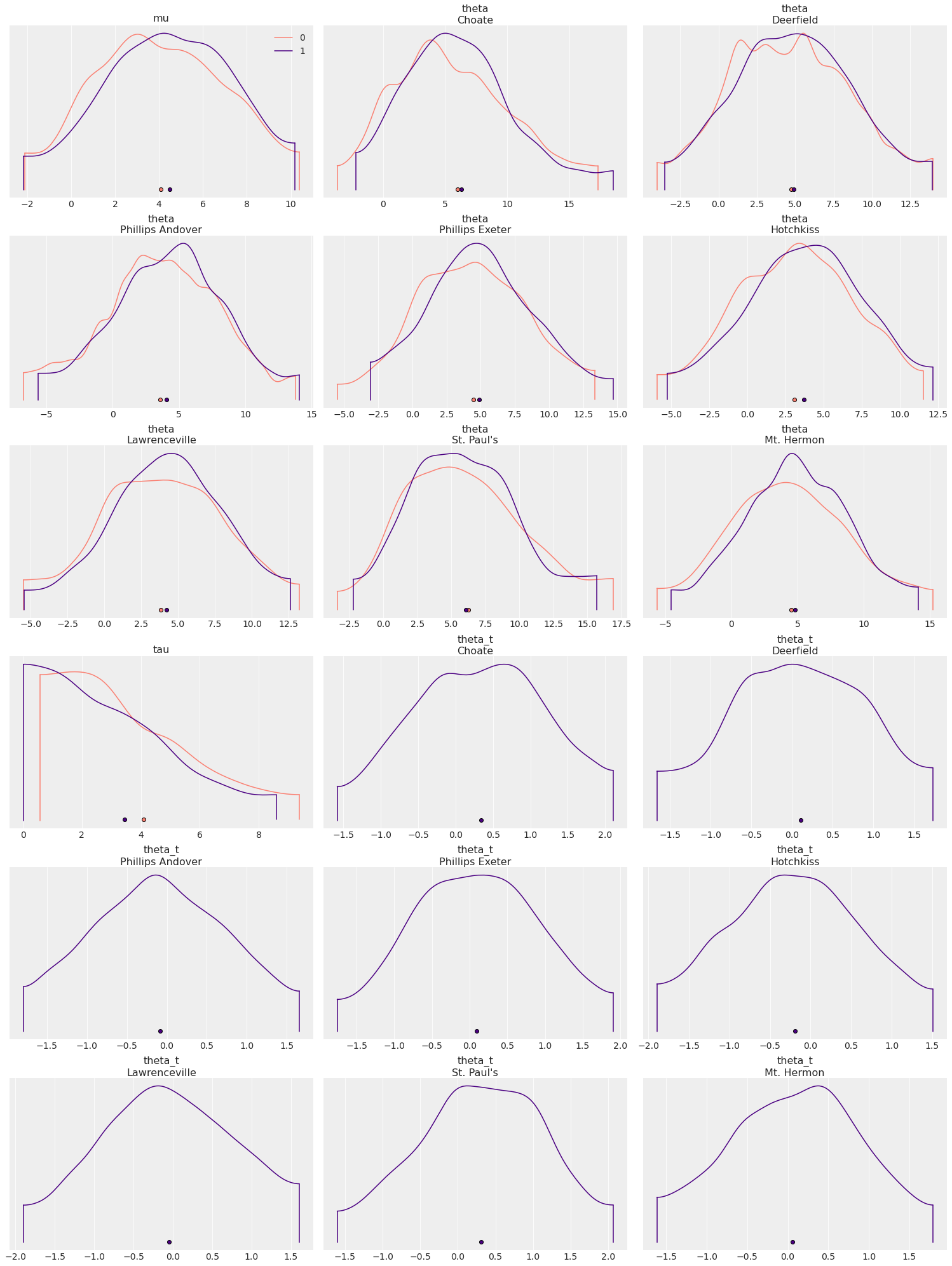
combine_dims dims can be used to generate the KDE of the distribution of theta
when combining all schools together.
az.plot_posterior(centered_eight, var_names=["mu", "theta"], combine_dims={"school"});
Warning
plot_pair also supports combine_dims argument, but it’s the users responsibility
to ensure the variables to be plotted have compatible dimensions when reducing
them pairwise.
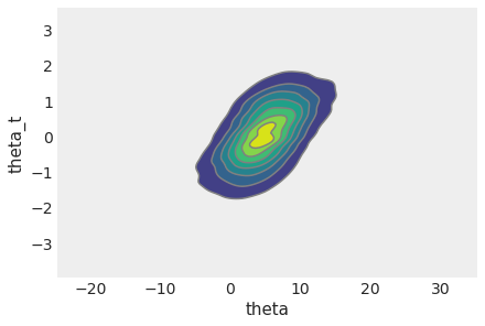
Both theta and theta_t have the school dimension, so we can use combine_dims
in plot_pair to generate their global 2d KDE.
az.plot_pair(
    non_centered_eight, var_names=["theta", "theta_t"], combine_dims={"school"}, kind="kde"
);
mu however does not, so trying to plot their combined distribution errors out:
az.plot_pair(non_centered_eight, var_names=["theta", "mu"], combine_dims={"school"});
---------------------------------------------------------------------------
ValueError                                Traceback (most recent call last)
Input In [17], in <cell line: 1>()
----> 1 az.plot_pair(non_centered_eight, var_names=["theta", "mu"], combine_dims={"school"})

File ~/checkouts/readthedocs.org/user_builds/arviz/envs/v0.12.1/lib/python3.8/site-packages/arviz/plots/pairplot.py:291, in plot_pair(data, group, var_names, filter_vars, combine_dims, coords, marginals, figsize, textsize, kind, gridsize, contour, plot_kwargs, fill_last, divergences, colorbar, labeller, ax, divergences_kwargs, scatter_kwargs, kde_kwargs, hexbin_kwargs, backend, backend_kwargs, marginal_kwargs, point_estimate, point_estimate_kwargs, point_estimate_marker_kwargs, reference_values, reference_values_kwargs, show)
    289 # TODO: Add backend kwargs
    290 plot = get_plotting_function("plot_pair", "pairplot", backend)
--> 291 ax = plot(**pairplot_kwargs)
    292 return ax

File ~/checkouts/readthedocs.org/user_builds/arviz/envs/v0.12.1/lib/python3.8/site-packages/arviz/plots/backends/matplotlib/pairplot.py:176, in plot_pair(ax, plotters, numvars, figsize, textsize, kind, scatter_kwargs, kde_kwargs, hexbin_kwargs, gridsize, colorbar, divergences, diverging_mask, divergences_kwargs, flat_var_names, backend_kwargs, marginal_kwargs, show, marginals, point_estimate, point_estimate_kwargs, point_estimate_marker_kwargs, reference_values, reference_values_kwargs)
    173         ax = np.atleast_2d(ax)[0, 0]
    175 if "scatter" in kind:
--> 176     ax.plot(x, y, **scatter_kwargs)
    177 if "kde" in kind:
    178     plot_kde(x, y, ax=ax, **kde_kwargs)

File ~/checkouts/readthedocs.org/user_builds/arviz/envs/v0.12.1/lib/python3.8/site-packages/matplotlib/axes/_axes.py:1632, in Axes.plot(self, scalex, scaley, data, *args, **kwargs)
   1390 """
   1391 Plot y versus x as lines and/or markers.
   1392
   (...)
   1629 (``'green'``) or hex strings (``'#008000'``).
   1630 """
   1631 kwargs = cbook.normalize_kwargs(kwargs, mlines.Line2D)
-> 1632 lines = [*self._get_lines(*args, data=data, **kwargs)]
   1633 for line in lines:
   1634     self.add_line(line)

File ~/checkouts/readthedocs.org/user_builds/arviz/envs/v0.12.1/lib/python3.8/site-packages/matplotlib/axes/_base.py:312, in _process_plot_var_args.__call__(self, data, *args, **kwargs)
    310     this += args[0],
    311     args = args[1:]
--> 312 yield from self._plot_args(this, kwargs)

File ~/checkouts/readthedocs.org/user_builds/arviz/envs/v0.12.1/lib/python3.8/site-packages/matplotlib/axes/_base.py:498, in _process_plot_var_args._plot_args(self, tup, kwargs, return_kwargs)
    495     self.axes.yaxis.update_units(y)
    497 if x.shape[0] != y.shape[0]:
--> 498     raise ValueError(f"x and y must have same first dimension, but "
    499                      f"have shapes {x.shape} and {y.shape}")
    500 if x.ndim > 2 or y.ndim > 2:
    501     raise ValueError(f"x and y can be no greater than 2D, but have "
    502                      f"shapes {x.shape} and {y.shape}")

ValueError: x and y must have same first dimension, but have shapes (16000,) and (2000,)
combine_dims can be used alongside combined, but it can’t be used to replace it.
When combined=True, ArviZ does extra processing in addition to adding
"chain" to combine_dims under the hood. Therefore:
az.plot_forest(
    centered_eight, var_names="theta", combined=True, combine_dims={"school"}
);
is not equivalent to:
az.plot_forest(
    centered_eight, var_names="theta", combine_dims={"chain", "school"}
);
hdi_prob#
Probability for the highest density interval (HDI).
Defaults to stats.hdi_prob rcParam.
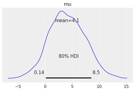
Plot the 80% HDI interval of simulated regression data using y argument:
az.plot_posterior(centered_eight, var_names="mu", hdi_prob=0.8);
grid#
Number of rows and columns. Defaults to None, the rows and columns are automatically inferred.
Plot variables in a 4x5 grid:
az.plot_density([centered_eight, non_centered_eight], grid=(4, 5));
figsize#
figsize is short for figure size, expressed as a tuple.
By default it is defined automatically.
az.plot_posterior(centered_eight, var_names=["mu", "tau"], figsize=(3, 6));
textsize#
Text size for labels, titles and lines.
By default it is autoscaled based on figsize.
az.plot_posterior(centered_eight, var_names="theta", coords=coords, textsize=30);
color or colors#
Color used for the main element or elements of the plot. It should be a valid matplotlib color, even if using the bokeh backend.
While both libraries use CSS colors as their base named colors,
matplotlib also supports theme based colors like C0 as well
as tableau and xkcd colors. ArviZ converts the provided colors
to hex RGB format using matplotlib before passing it to either
plotting backend.
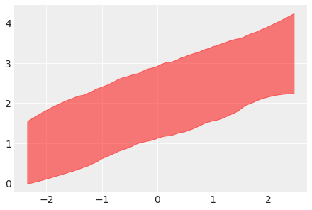
Plot the HDI interval of simulated regression data using y argument, in red:
az.plot_hdi(x_data, y_data, color="red");
colors behaves like color but it takes an iterable of colors instead
of a single color. The number of colors to be provided is defined by
the models being compared (like in plot_density) of by the number
of different quantities being plotted (like in plot_ppc).
Warning
In plot_elpd() and plot_khat(), where scatter plots are generated with
one dot per observation, color can also take an array_like of colors, one per dot.
There are examples in their respective docstrings.
az.plot_density([centered_eight, non_centered_eight], colors=["salmon", "indigo"]);
legend#
Show a legend with the color encoded model information. Defaults to True, if there are multiple models.
List with names for the models in the list of data. Useful when plotting more that one dataset.
ax#
matplotlib.axes.Axes or bokeh.plotting.Figure.
backend#
Select plotting backend {“matplotlib”,”bokeh”}. Defaults to “matplotlib”.
backend_kwargs#
These are kwargs specific to the backend being used, passed to matplotlib.pyplot.subplots or bokeh.plotting.figure. For additional documentation check the plotting method of the backend.
show#
Call backend show function.