Plotting with Matplotlib#
Matplotlib is the default backend for ArviZ. Although most of the functions in the plot module work seamlessly with any backend, some advanced plots may require the use of backend specific features. In this guide, advanced plotting with Matplotlib will be covered.
This page can be downloaded as a Python script
or as a Jupyter notebook.
import arviz as az
import matplotlib.pyplot as plt
import numpy as np

az.style.use("arviz-darkgrid")
Customizing plots#
Using backend_kwargs#
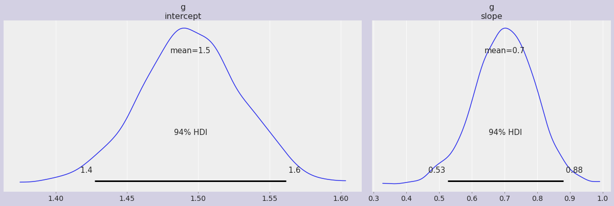
The backend_kwargs argument can be very useful for some specific configuration. That is parameters available in matplotlib.pyplot.subplots(), which includes add_subplot() and GridSpec through subplot_kw and gridspec_kw respectively. As the options available depends on the backend, this parameter is not as flexible as creating custom axes.
As an example, the following code changes the facecolor from figure() and the width_ratios in the grid layout.
# load data
data = az.load_arviz_data('radon')
az.plot_posterior(
    data,
    var_names=["g"],
    backend_kwargs={
        "facecolor": "#d3d0e3",
        "gridspec_kw": {
            "width_ratios": [6,4]}});
Caution
The parameters ncol and nrows from matplotlib.pyplot.subplots() should not be set using the backend_kwargs parameter. Instead, use the param grid
The parameter show#
The parameter show calls matplotlib.pyplot.show() if set to True. If show is not set, it will take the value from the rcParam plot.matplotlib.show which defaults to False.
Note
There are some Matplotlib backends like the inline (default) Jupyter backend that show the plot even if plt.show is not called. In such cases, plots will be shown automatically even if show=False.
Defining custom axes#
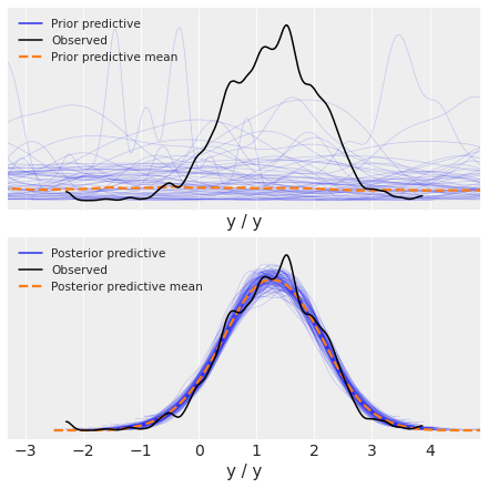
The ax argument of any plot function allows to use created axes manually. In the example, this parameter allows to arrange 2 different plots in a grid, set limit to the x axis and share the axes between the two plots.
# load data
observed_data = data.observed_data.y.values
# create axes
_, ax = plt.subplots(2, 1, sharex=True, sharey=True, figsize=(6, 6))
ax[0].set_xlim(xmin=observed_data.min() - 1, xmax=observed_data.max() + 1)
# plot
az.plot_ppc(data, group="prior", num_pp_samples=100, ax=ax[0])
az.plot_ppc(data, group="posterior", num_pp_samples=100, ax=ax[1]);
Extending ArviZ-Matplotlib plots#
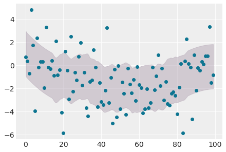
As an Arviz plot returns an Axes object, different Matplotlib plots can be added to a plot generated with Arviz:
# load data
data = az.load_arviz_data('regression1d')
X = data.observed_data.y_dim_0
Y = data.observed_data.y
y_pp = data.posterior_predictive.y
# plot
ax = az.plot_hdi(X, y_pp, color="#b5a7b6")
ax.scatter(X, Y, c="#0d7591");
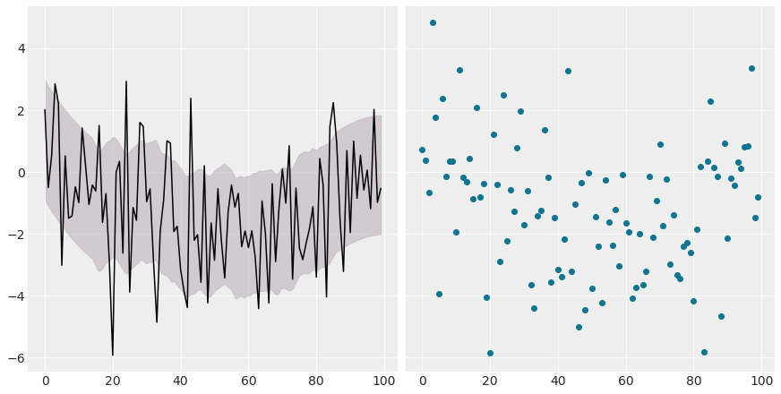
Similarly, custom axes allow to display Arviz and Matplotlib plots in the same grid. In this example, the plot in ax1 has an Arviz plot modified with a Matplotlib plot and the ax2 has a scatter created using Matplotlib.
# create axes
_, (ax1, ax2) = plt.subplots(1, 2, figsize=(12, 6), sharey=True)
# plot ax1
az.plot_hdi(X, y_pp, color="#b5a7b6", ax=ax1)
ax1.plot(X, y_pp.mean(axis=(0, 1)), c="black")
# plot ax2
ax2.scatter(X, Y, c="#0d7591");