ArviZ Quickstart#
import arviz as az
import numpy as np
ArviZ style sheets#
# ArviZ ships with style sheets!
az.style.use("arviz-darkgrid")
Feel free to check the examples of style sheets here.
Get started with plotting#
ArviZ is designed to be used with libraries like PyStan and PyMC3, but works fine with raw NumPy arrays.
rng = np.random.default_rng()
az.plot_posterior(rng.normal(size=100_000));
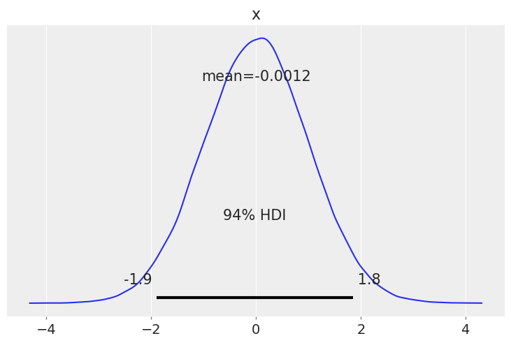
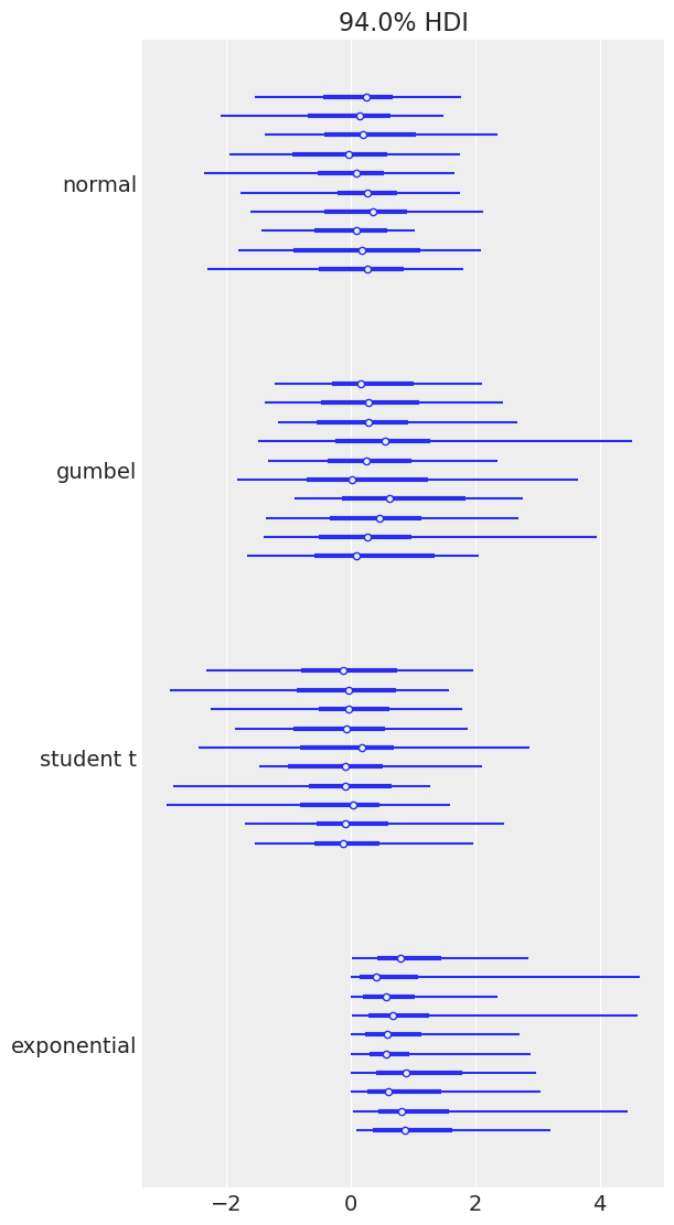
Plotting a dictionary of arrays, ArviZ will interpret each key as the name of a different random variable. Each row of an array is treated as an independent series of draws from the variable, called a chain. Below, we have 10 chains of 50 draws, each for four different distributions.
size = (10, 50)
az.plot_forest(
    {
        "normal": rng.normal(size=size),
        "gumbel": rng.gumbel(size=size),
        "student t": rng.standard_t(df=6, size=size),
        "exponential": rng.exponential(size=size),
    }
);
ArviZ rcParams#
You may have noticed that for both plot_posterior() and plot_forest(), the Highest Density Interval (HDI) is 94%, which you may find weird at first. This particular value is a friendly reminder of the arbitrary nature of choosing any single value without further justification, including common values like 95%, 50% and even our own default, 94%. ArviZ includes default values for a few parameters, you can access them with az.rcParams. To change the default HDI value to let’s say 90% you can do:
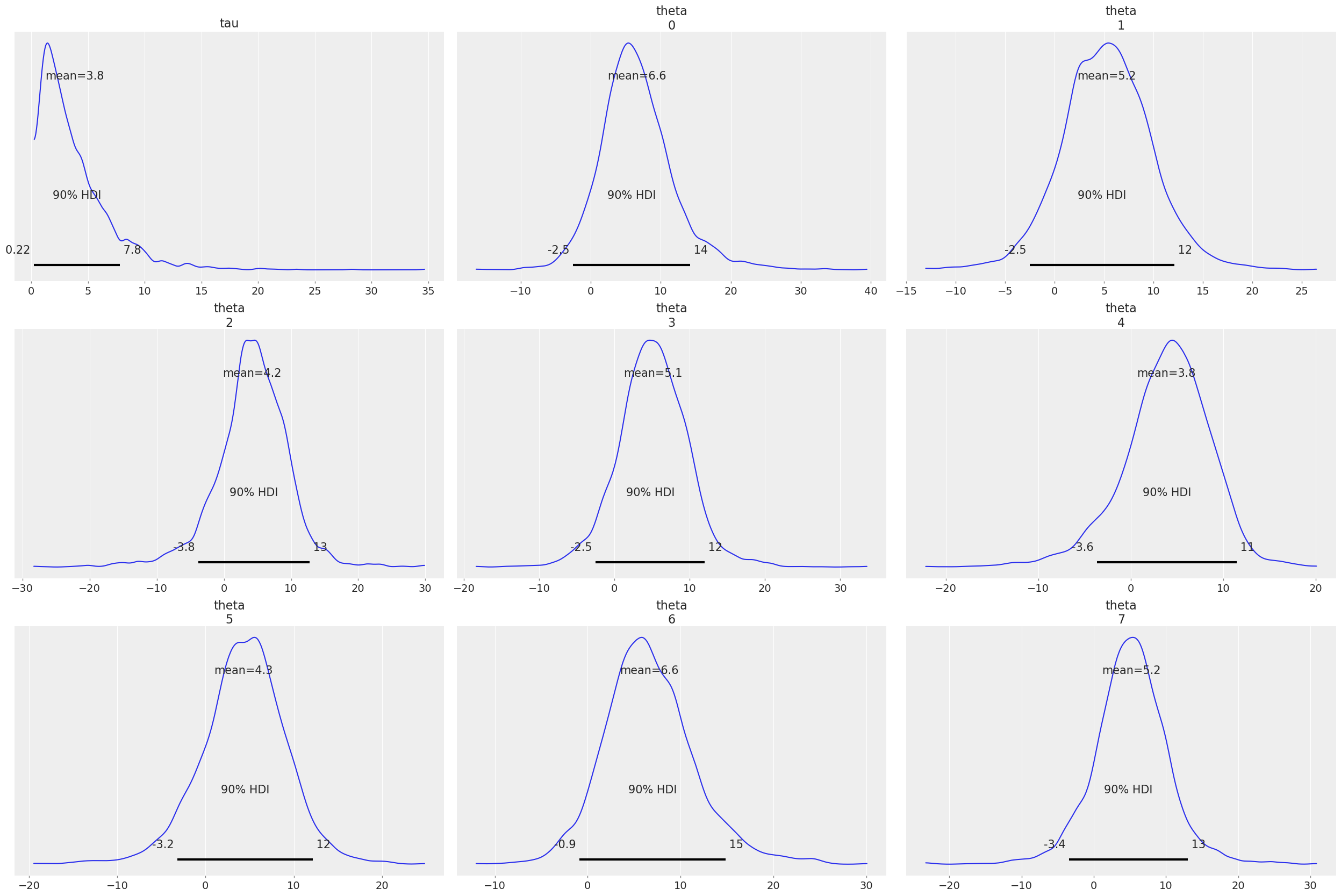
az.rcParams["stats.hdi_prob"] = 0.90
PyMC integration#
ArviZ integrates with PyMC. In fact, the object returned by default by most PyMC sampling methods is the arviz.InferenceData object.
Therefore, we only need to define a model, sample from it and we can use the result with ArviZ straight away.
import pymc as pm
with pm.Model(coords={"school": schools}) as centered_eight:
    mu = pm.Normal("mu", mu=0, sigma=5)
    tau = pm.HalfCauchy("tau", beta=5)
    theta = pm.Normal("theta", mu=mu, sigma=tau, dims="school")
    pm.Normal("obs", mu=theta, sigma=sigma, observed=y, dims="school")

    # This pattern can be useful in PyMC
    idata = pm.sample_prior_predictive()
    idata.extend(pm.sample())
    pm.sample_posterior_predictive(idata, extend_inferencedata=True)
Sampling: [mu, obs, tau, theta]
Auto-assigning NUTS sampler...
Initializing NUTS using jitter+adapt_diag...
Multiprocess sampling (4 chains in 4 jobs)
NUTS: [mu, tau, theta]
Sampling 4 chains for 1_000 tune and 1_000 draw iterations (4_000 + 4_000 draws total) took 6 seconds.
The rhat statistic is larger than 1.01 for some parameters. This indicates problems during sampling. See https://arxiv.org/abs/1903.08008 for details
The effective sample size per chain is smaller than 100 for some parameters.  A higher number is needed for reliable rhat and ess computation. See https://arxiv.org/abs/1903.08008 for details
There were 84 divergences after tuning. Increase `target_accept` or reparameterize.
Sampling: [obs]
Here we have combined the outputs of prior sampling, MCMC sampling to obtain the posterior samples and posterior predictive samples into a single InferenceData, the main ArviZ data structure.
The more groups it has contains the more powerful analyses it can perform. You can check the InferenceData structure specification here.
Tip
By default, PyMC does not compute the pointwise log likelihood values, which are needed for model comparison with WAIC or PSIS-LOO-CV.
Use idata_kwargs={"log_likelihood": True} to have it computed right after sampling for you. Alternatively, you can also use
pymc.compute_log_likelihood() before calling compare(), loo(), waic() or loo_pit()
idata
-
<xarray.Dataset> Dimensions: (chain: 4, draw: 1000, school: 8) Coordinates: * chain (chain) int64 0 1 2 3 * draw (draw) int64 0 1 2 3 4 5 6 7 8 ... 992 993 994 995 996 997 998 999 * school (school) <U16 'Choate' 'Deerfield' ... "St. Paul's" 'Mt. Hermon' Data variables: mu (chain, draw) float64 10.02 7.399 6.104 1.803 ... 1.041 12.6 10.12 theta (chain, draw, school) float64 8.304 4.128 12.45 ... 12.92 10.8 tau (chain, draw) float64 3.041 3.737 3.529 1.581 ... 3.22 1.696 2.607 Attributes: created_at: 2023-12-21T18:42:25.932752 arviz_version: 0.17.0.dev0 inference_library: pymc inference_library_version: 5.10.2 sampling_time: 5.5613462924957275 tuning_steps: 1000 -
<xarray.Dataset> Dimensions: (chain: 4, draw: 1000, school: 8) Coordinates: * chain (chain) int64 0 1 2 3 * draw (draw) int64 0 1 2 3 4 5 6 7 8 ... 992 993 994 995 996 997 998 999 * school (school) <U16 'Choate' 'Deerfield' ... "St. Paul's" 'Mt. Hermon' Data variables: obs (chain, draw, school) float64 -4.287 -7.086 3.44 ... 11.22 39.41 Attributes: created_at: 2023-12-21T18:42:27.486051 arviz_version: 0.17.0.dev0 inference_library: pymc inference_library_version: 5.10.2 -
<xarray.Dataset> Dimensions: (chain: 4, draw: 1000) Coordinates: * chain (chain) int64 0 1 2 3 * draw (draw) int64 0 1 2 3 4 5 ... 994 995 996 997 998 999 Data variables: (12/17) energy (chain, draw) float64 57.32 60.94 ... 61.22 58.55 step_size (chain, draw) float64 0.264 0.264 ... 0.2667 0.2667 index_in_trajectory (chain, draw) int64 2 -4 -5 5 3 -4 ... 1 0 -8 2 -10 6 energy_error (chain, draw) float64 0.1952 0.251 ... -0.1325 0.279 tree_depth (chain, draw) int64 3 3 4 4 4 3 4 4 ... 2 4 3 4 3 5 3 process_time_diff (chain, draw) float64 0.001172 0.001172 ... 0.001192 ... ... diverging (chain, draw) bool False False False ... False False acceptance_rate (chain, draw) float64 0.8216 0.7868 ... 0.9907 0.842 n_steps (chain, draw) float64 7.0 7.0 15.0 ... 7.0 23.0 7.0 lp (chain, draw) float64 -55.39 -55.34 ... -55.68 -51.57 step_size_bar (chain, draw) float64 0.2845 0.2845 ... 0.2817 0.2817 perf_counter_start (chain, draw) float64 1.286e+04 ... 1.286e+04 Attributes: created_at: 2023-12-21T18:42:25.944471 arviz_version: 0.17.0.dev0 inference_library: pymc inference_library_version: 5.10.2 sampling_time: 5.5613462924957275 tuning_steps: 1000 -
<xarray.Dataset> Dimensions: (chain: 1, draw: 500, school: 8) Coordinates: * chain (chain) int64 0 * draw (draw) int64 0 1 2 3 4 5 6 7 8 ... 492 493 494 495 496 497 498 499 * school (school) <U16 'Choate' 'Deerfield' ... "St. Paul's" 'Mt. Hermon' Data variables: theta (chain, draw, school) float64 52.13 -71.41 148.5 ... 1.115 6.39 tau (chain, draw) float64 120.4 7.113 1.983 2.866 ... 8.423 6.926 12.31 mu (chain, draw) float64 -2.798 1.822 -4.905 ... -1.888 -4.516 1.978 Attributes: created_at: 2023-12-21T18:42:18.246297 arviz_version: 0.17.0.dev0 inference_library: pymc inference_library_version: 5.10.2 -
<xarray.Dataset> Dimensions: (chain: 1, draw: 500, school: 8) Coordinates: * chain (chain) int64 0 * draw (draw) int64 0 1 2 3 4 5 6 7 8 ... 492 493 494 495 496 497 498 499 * school (school) <U16 'Choate' 'Deerfield' ... "St. Paul's" 'Mt. Hermon' Data variables: obs (chain, draw, school) float64 78.06 -75.96 125.8 ... 2.925 19.95 Attributes: created_at: 2023-12-21T18:42:18.248182 arviz_version: 0.17.0.dev0 inference_library: pymc inference_library_version: 5.10.2 -
<xarray.Dataset>
Dimensions:  (school: 8)
Coordinates:
  * school   (school) <U16 'Choate' 'Deerfield' ... "St. Paul's" 'Mt. Hermon'
Data variables:
    obs      (school) float64 28.0 8.0 -3.0 7.0 -1.0 1.0 18.0 12.0
Attributes:
    created_at:                 2023-12-21T18:42:18.248964
    arviz_version:              0.17.0.dev0
    inference_library:          pymc
    inference_library_version:  5.10.2
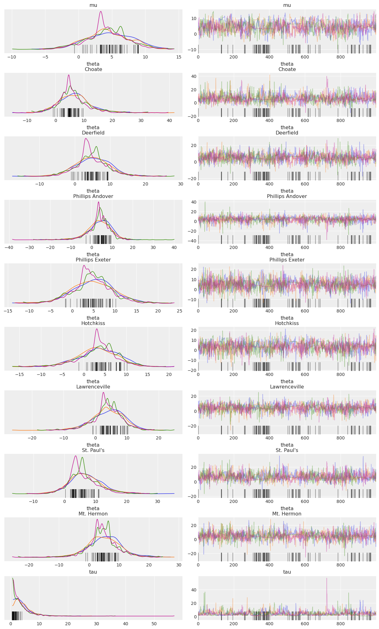
Below is a “trace plot”, a common visualization to check MCMC output and assess convergence. Note that the labeling information we included in the PyMC model via the coords and dims arguments is kept and added to the plot (it is also available in the InferenceData HTML representation above):
az.plot_trace(idata, compact=False);
CmdStanPy integration#
ArviZ also has first class support for CmdStanPy. After creating and sampling a CmdStanPy model:
from cmdstanpy import CmdStanModel
model = CmdStanModel(stan_file="schools.stan")
/home/oriol/bin/miniforge3/envs/general/lib/python3.11/site-packages/tqdm/auto.py:21: TqdmWarning: IProgress not found. Please update jupyter and ipywidgets. See https://ipywidgets.readthedocs.io/en/stable/user_install.html
  from .autonotebook import tqdm as notebook_tqdm
fit = model.sample(data="schools.json")
19:42:30 - cmdstanpy - INFO - CmdStan start processing
chain 1 |                                                                       | 00:00 Status
chain 2 |                                                                       | 00:00 Status

chain 3 |                                                                       | 00:00 Status


chain 4 |                                                                       | 00:00 Status

chain 3 |███████████████████████████████     | 00:00 Iteration: 1600 / 2000 [ 80%]  (Sampling)


chain 1 |███████████████████████████████████████████████████████████| 00:00 Sampling completed

chain 2 |███████████████████████████████████████████████████████████| 00:00 Sampling completed
chain 3 |███████████████████████████████████████████████████████████| 00:00 Sampling completed
chain 4 |███████████████████████████████████████████████████████████| 00:00 Sampling completed
19:42:30 - cmdstanpy - INFO - CmdStan done processing.
19:42:30 - cmdstanpy - WARNING - Some chains may have failed to converge.
	Chain 1 had 27 divergent transitions (2.7%)
	Chain 2 had 9 divergent transitions (0.9%)
	Chain 3 had 4 divergent transitions (0.4%)
	Chain 4 had 20 divergent transitions (2.0%)
	Use the "diagnose()" method on the CmdStanMCMC object to see further information.
The result can be used for plotting with ArviZ directly:
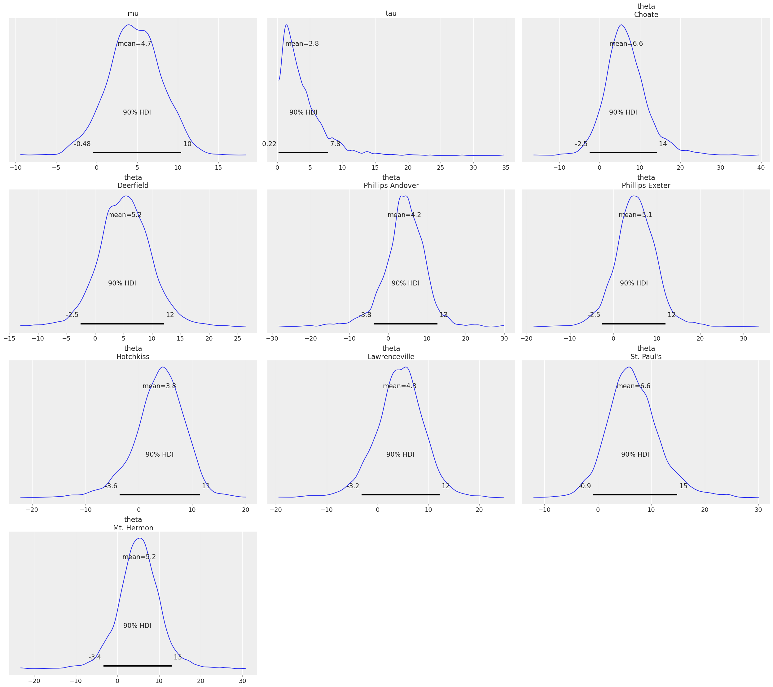
az.plot_posterior(fit, var_names=["tau", "theta"]);
To make the most out of ArviZ however, it is recommended to convert the results to InferenceData. This will ensure all variables are assigned to the right groups and also gives you the option of labeling the data.
Tip
If ArviZ finds any variable names log_lik in the CmdStanPy output, it will interpret them as the pointwise log likelihood values,
in line with the Stan conventions used by the R libraries.
idata = az.from_cmdstanpy(
    fit,
    posterior_predictive="y_hat",
    dims={"y_hat": ["school"], "theta": ["school"]},
    coords={"school": schools}
)
az.plot_posterior(idata, var_names=["tau", "theta"]);
See also
creating_InferenceData working_with_InferenceData