arviz.plot_dist#
- arviz.plot_dist(values, values2=None, color='C0', kind='auto', cumulative=False, label=None, rotated=False, rug=False, bw='default', quantiles=None, contour=True, fill_last=True, figsize=None, textsize=None, plot_kwargs=None, fill_kwargs=None, rug_kwargs=None, contour_kwargs=None, contourf_kwargs=None, pcolormesh_kwargs=None, hist_kwargs=None, is_circular=False, ax=None, backend=None, backend_kwargs=None, show=None, **kwargs)[source]#
Plot distribution as histogram or kernel density estimates.
By default continuous variables are plotted using KDEs and discrete ones using histograms
- Parameters:
- valuesarray_like
Values to plot from an unknown continuous or discrete distribution.
- values2array_like, optional
Values to plot. If present, a 2D KDE or a hexbin will be estimated.
- color
str valid matplotlib color.
- kind
str, default “auto” By default (“auto”) continuous variables will use the kind defined by rcParam
plot.density_kindand discrete ones will use histograms. To override this use “hist” to plot histograms and “kde” for KDEs.- cumulativebool, default
False If true plot the estimated cumulative distribution function. Defaults to False. Ignored for 2D KDE.
- label
str Text to include as part of the legend.
- rotatedbool, default
False Whether to rotate the 1D KDE plot 90 degrees.
- rugbool, default
False Add a rug plot for a specific subset of values. Ignored for 2D KDE.
- bw
floatorstr, optional If numeric, indicates the bandwidth and must be positive. If str, indicates the method to estimate the bandwidth and must be one of “scott”, “silverman”, “isj” or “experimental” when
is_circularis False and “taylor” (for now) whenis_circularis True. Defaults to “experimental” when variable is not circular and “taylor” when it is.- quantiles
list, optional Quantiles in ascending order used to segment the KDE. Use [.25, .5, .75] for quartiles.
- contourbool, default
True If True plot the 2D KDE using contours, otherwise plot a smooth 2D KDE.
- fill_lastbool, default
True If True fill the last contour of the 2D KDE plot.
- figsize(
float,float), optional Figure size. If
Noneit will be defined automatically.- textsize
float, optional Text size scaling factor for labels, titles and lines. If
Noneit will be autoscaled based onfigsize. Not implemented for bokeh backend.- plot_kwargs
dict Keywords passed to the pdf line of a 1D KDE. Passed to
arviz.plot_kde()asplot_kwargs.- fill_kwargs
dict Keywords passed to the fill under the line (use fill_kwargs={‘alpha’: 0} to disable fill). Ignored for 2D KDE. Passed to
arviz.plot_kde()asfill_kwargs.- rug_kwargs
dict Keywords passed to the rug plot. Ignored if
rug=Falseor for 2D KDE Usespacekeyword (float) to control the position of the rugplot. The larger this number the lower the rugplot. Passed toarviz.plot_kde()asrug_kwargs.- contour_kwargs
dict Keywords passed to the contourplot. Ignored for 1D KDE.
- contourf_kwargs
dict Keywords passed to
matplotlib.axes.Axes.contourf(). Ignored for 1D KDE.- pcolormesh_kwargs
dict Keywords passed to
matplotlib.axes.Axes.pcolormesh(). Ignored for 1D KDE.- hist_kwargs
dict Keyword arguments used to customize the histogram. Ignored when plotting a KDE. They are passed to
matplotlib.axes.Axes.hist()if using matplotlib, or tobokeh.plotting.figure.quad()if using bokeh. In bokeh case, the following extra keywords are also supported:color: replaces thefill_colorandline_colorof thequadmethodbins: taken fromhist_kwargsand passed tonumpy.histogram()insteaddensity: normalize histogram to represent a probability density function, Defaults toTruecumulative: plot the cumulative counts. Defaults toFalse.
- is_circular{
False,True, “radians”, “degrees”}, defaultFalse Select input type {“radians”, “degrees”} for circular histogram or KDE plot. If True, default input type is “radians”. When this argument is present, it interprets the values passed are from a circular variable measured in radians and a circular KDE is used. Inputs in “degrees” will undergo an internal conversion to radians. Only valid for 1D KDE.
- ax
matplotlib AxesorBokeh Figure, optional Matplotlib or bokeh targets on which to plot. If not supplied, Arviz will create its own plot area (and return it).
- backend{“matplotlib”, “bokeh”}, default “matplotlib”
Select plotting backend.
- backend_kwargs :dict, optional
These are kwargs specific to the backend being used, passed to
matplotlib.pyplot.subplots()orbokeh.plotting.figure. For additional documentation check the plotting method of the backend.- showbool, optional
Call backend show function.
- Returns:
- axes
matplotlibaxesorbokehfigure
- axes
See also
plot_posteriorPlot Posterior densities in the style of John K. Kruschke’s book.
plot_densityGenerate KDE plots for continuous variables and histograms for discrete ones.
plot_kde1D or 2D KDE plot taking into account boundary conditions.
Examples
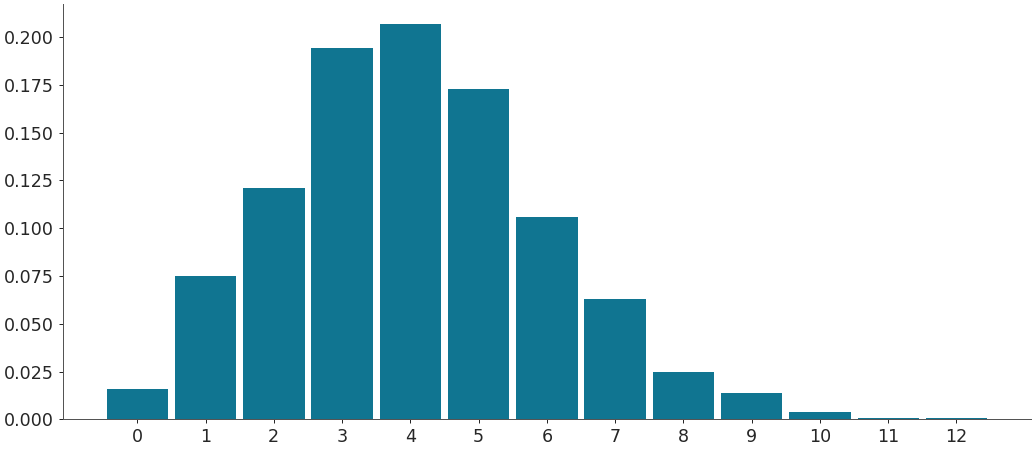
Plot an integer distribution
>>> import numpy as np
>>> import arviz as az
>>> a = np.random.poisson(4, 1000)
>>> az.plot_dist(a)
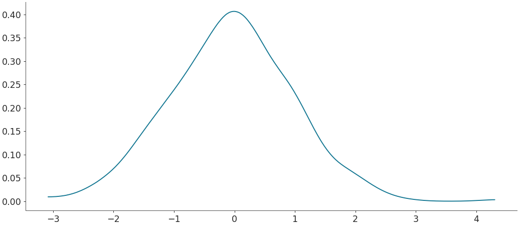
Plot a continuous distribution
>>> b = np.random.normal(0, 1, 1000)
>>> az.plot_dist(b)
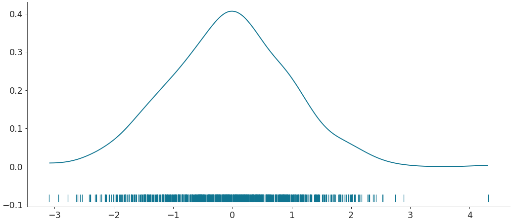
Add a rug under the Gaussian distribution
>>> az.plot_dist(b, rug=True)
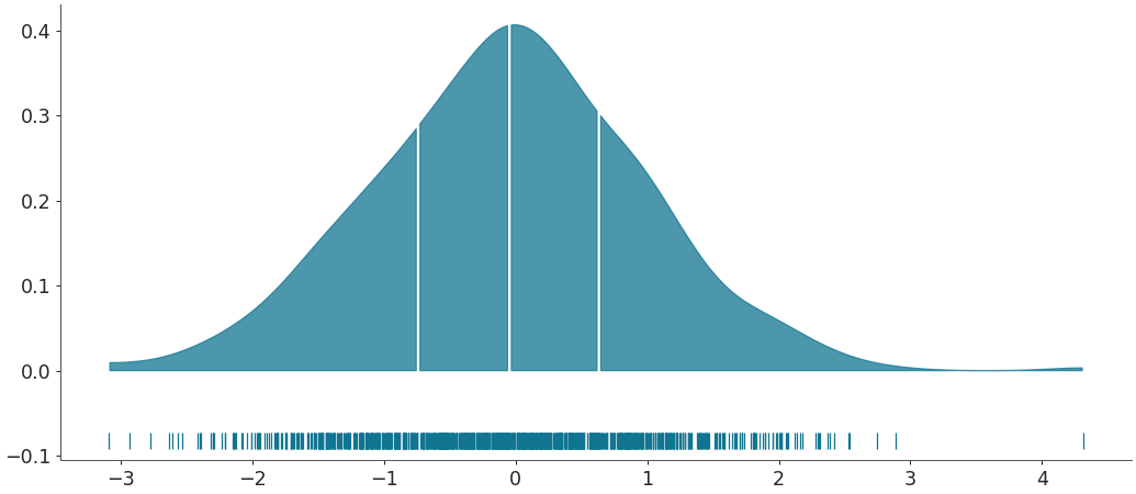
Segment into quantiles
>>> az.plot_dist(b, rug=True, quantiles=[.25, .5, .75])
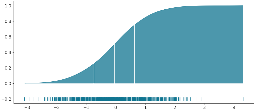
Plot as the cumulative distribution
>>> az.plot_dist(b, rug=True, quantiles=[.25, .5, .75], cumulative=True)