arviz.plot_bf#
- arviz.plot_bf(idata, var_name, prior=None, ref_val=0, colors=('C0', 'C1'), figsize=None, textsize=None, hist_kwargs=None, plot_kwargs=None, ax=None, backend=None, backend_kwargs=None, show=None)[source]#
Approximated Bayes Factor for comparing hypothesis of two nested models.
The Bayes factor is estimated by comparing a model (H1) against a model in which the parameter of interest has been restricted to be a point-null (H0). This computation assumes the models are nested and thus H0 is a special case of H1.
- Parameters:
- idata
InferenceData Any object that can be converted to an
arviz.InferenceDataobject Refer to documentation ofarviz.convert_to_dataset()for details.- var_name
str, optional Name of variable we want to test.
- prior
numpy.array, optional In case we want to use different prior, for example for sensitivity analysis.
- ref_val
int, default 0 Point-null for Bayes factor estimation.
- colors
tuple, default (‘C0’, ‘C1’) Tuple of valid Matplotlib colors. First element for the prior, second for the posterior.
- figsize(
float,float), optional Figure size. If
Noneit will be defined automatically.- textsize
float, optional Text size scaling factor for labels, titles and lines. If
Noneit will be auto scaled based onfigsize.- plot_kwargs
dict, optional Additional keywords passed to
matplotlib.pyplot.plot().- hist_kwargs
dict, optional Additional keywords passed to
arviz.plot_dist(). Only works for discrete variables.- ax
axes, optional matplotlib.axes.Axesorbokeh.plotting.Figure.- backend{“matplotlib”, “bokeh”}, default “matplotlib”
Select plotting backend.
- backend_kwargs
dict, optional These are kwargs specific to the backend being used, passed to
matplotlib.pyplot.subplots()orbokeh.plotting.figure. For additional documentation check the plotting method of the backend.- showbool, optional
Call backend show function.
- idata
- Returns:
- dict
AdictionarywithBF10(BayesFactor10 (H1/H0ratio),andBF01(H0/H1ratio). - axes
matplotlib AxesorBokeh Figure
- dict
Notes
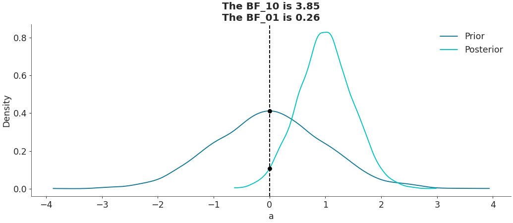
The bayes Factor is approximated as the Savage-Dickey density ratio algorithm presented in [1].
References
[1]Heck, D., 2019. A caveat on the Savage-Dickey density ratio: The case of computing Bayes factors for regression parameters.
Examples
Moderate evidence indicating that the parameter “a” is different from zero.
>>> import numpy as np
>>> import arviz as az
>>> idata = az.from_dict(posterior={"a":np.random.normal(1, 0.5, 5000)},
...     prior={"a":np.random.normal(0, 1, 5000)})
>>> az.plot_bf(idata, var_name="a", ref_val=0)