arviz.plot_ecdf

arviz.plot_ecdf(values, values2=None, cdf=None, difference=False, pit=False, confidence_bands=None, pointwise=False, npoints=100, num_trials=500, fpr=0.05, figsize=None, fill_band=True, plot_kwargs=None, fill_kwargs=None, plot_outline_kwargs=None, ax=None, show=None, backend=None, backend_kwargs=None, **kwargs)

Plot ECDF or ECDF-Difference Plot with Confidence bands.

This plot uses the simulated based algorithm presented in the paper “Graphical Test for Discrete Uniformity and its Applications in Goodness of Fit Evaluation and Multiple Sample Comparison” [1].

Parameters

valuesarray-like

Values to plot from an unknown continuous or discrete distribution

values2array-like, optional

Values to compare to the original sample

cdffunction, optional

Cumulative distribution function of the distribution to compare the original sample to

differencebool, optional, Defaults False

If true then plot ECDF-difference plot otherwise ECDF plot

pitbool, optional

If True plots the ECDF or ECDF-diff of PIT of sample

confidence_bandsbool, optional, Defaults True

If True plots the simultaneous or pointwise confidence bands with 1 - fpr confidence level

pointwisebool, optional, Defaults False

If True plots pointwise confidence bands otherwise simultaneous bands

npointsint, optional, Defaults 100

This denotes the granularity size of our plot i.e the number of evaluation points for our ecdf or ecdf-difference plot

num_trialsint, optional, Defaults 500

The number of random ECDFs to generate to construct simultaneous confidence bands

fprfloat, optional, Defaults 0.05

The type I error rate s.t 1 - fpr denotes the confidence level of bands

figsizetuple, optional

Figure size. If None it will be defined automatically.

fill_bandbool, optional

Use fill_between to mark the area inside the credible interval. Otherwise, plot the border lines.

plot_kwargsdict, optional

Additional kwargs passed to matplotlib.pyplot.step() or bokeh:bokeh.plotting.Figure.step()

fill_kwargsdict, optional

Additional kwargs passed to matplotlib.pyplot.fill_between() or bokeh:bokeh.plotting.Figure.varea()

plot_outline_kwargsdict, optional

Additional kwargs passed to matplotlib.axes.Axes.plot() or bokeh:bokeh.plotting.Figure.line()

axaxes, optional

Matplotlib axes or bokeh figures.

showbool, optional

Call backend show function.

backendstr, optional

Select plotting backend {“matplotlib”,”bokeh”}. Default “matplotlib”.

backend_kwargsdict, optional

These are kwargs specific to the backend being used, passed to matplotlib.pyplot.subplots() or bokeh:bokeh.plotting.figure().

Returns

axesmatplotlib axes or bokeh figures

References

1

Säilynoja, T., Bürkner, P.C. and Vehtari, A., 2021. Graphical Test for Discrete Uniformity and its Applications in Goodness of Fit Evaluation and Multiple Sample Comparison. arXiv preprint arXiv:2103.10522.

Examples

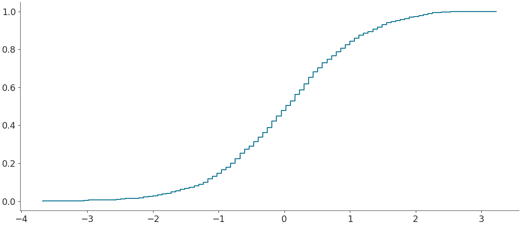
Plot ecdf plot for a given sample

>>> import arviz as az
>>> from scipy.stats import uniform, binom, norm

>>> sample = norm(0,1).rvs(1000)
>>> az.plot_ecdf(sample)

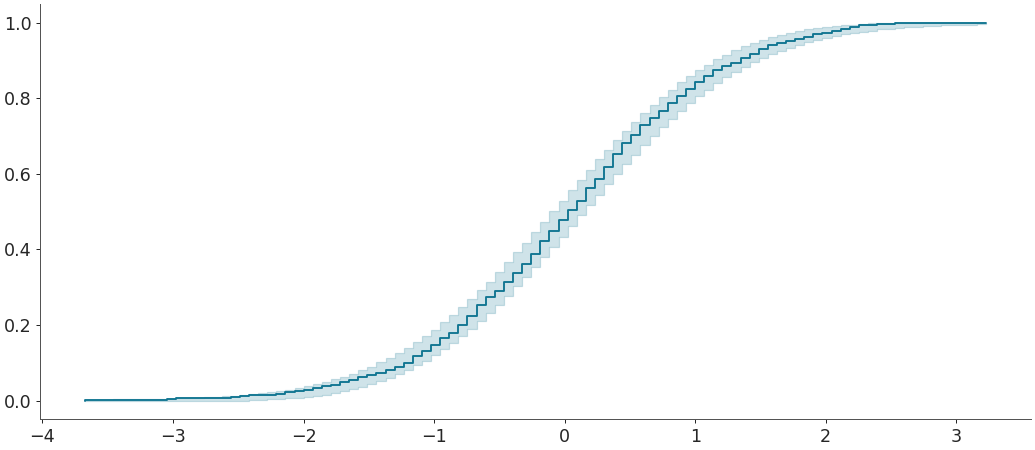
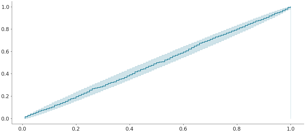
Plot ecdf plot with confidence bands for comparing a given sample w.r.t a given distribution

>>> distribution = norm(0,1)
>>> az.plot_ecdf(sample, cdf = distribution.cdf, confidence_bands = True)

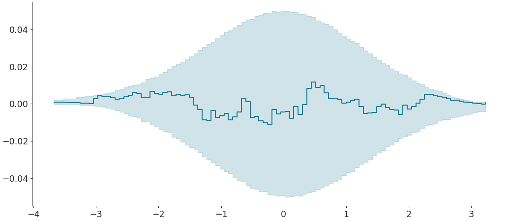
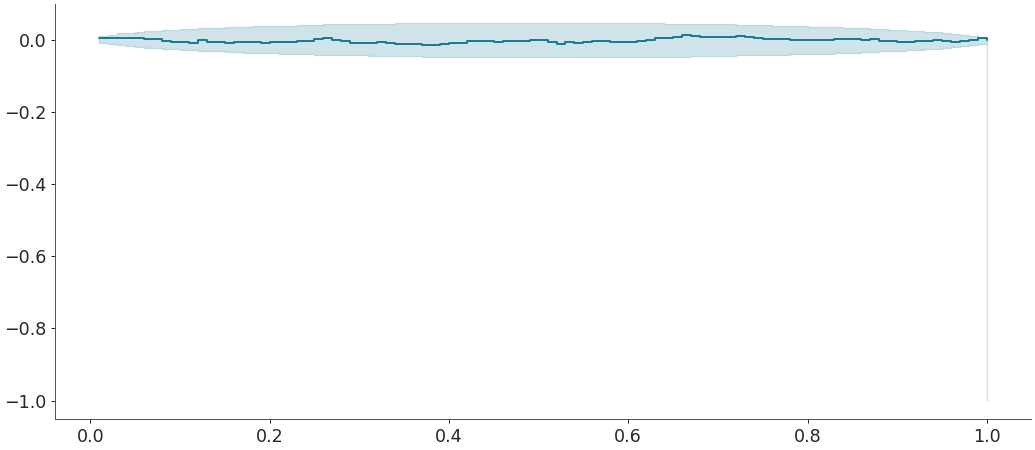
Plot ecdf-difference plot with confidence bands for comparing a given sample w.r.t a given distribution

>>> az.plot_ecdf(sample, cdf = distribution.cdf,
>>>              confidence_bands = True, difference = True)

Plot ecdf plot with confidence bands for PIT of sample for comparing a given sample w.r.t a given distribution

>>> az.plot_ecdf(sample, cdf = distribution.cdf,
>>>              confidence_bands = True, pit = True)

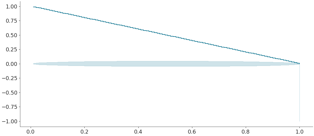
Plot ecdf-difference plot with confidence bands for PIT of sample for comparing a given sample w.r.t a given distribution

>>> az.plot_ecdf(sample, cdf = distribution.cdf,
>>>              confidence_bands = True, difference = True, pit = True)

You could also plot the above w.r.t another sample rather than a given distribution. For eg: Plot ecdf-difference plot with confidence bands for PIT of sample for comparing a given sample w.r.t a given sample

>>> sample2 = norm(0,1).rvs(5000)
>>> az.plot_ecdf(sample, sample2, confidence_bands = True, difference = True, pit = True)